Statistics in Ophthalmic Clinical Research
Argye Hillis
WHY STATISTICS?
For centuries, medical knowledge accumulated without benefit of statistics. Even today, clinical experience is the sine qua non of ophthalmology, and certain astute clinicians seem to have an uncanny ability to perceive and describe clinical processes by some intuitive strategy that belies formalization. However, such talent is rare and even those who possess it find an understanding of basic statistical concepts important for two reasons: objectivity and communication. Objectivity is important because we all are inclined to see what we want to see. Awareness of the danger is no protection—it may simply lead to “leaning over backward” in the other direction. Ophthalmologists are becoming increasingly demanding of scientific evidence on which to base clinical decisions. Properly employed statistical methods assist in determining just what the data say and how certain we can be of the message. Like any good language, statistics is also a tool for communication. The ophthalmologist with a background in statistics can present findings convincingly and is able to understand and evaluate the findings of others.
GETTING STARTED
Every field has its own technical jargon. Statistics is no exception. One barrier to communication with statisticians is the fact that certain common English words are used as technical terms with meanings quite different from common usage. For example, in statistics the words random, significant, and bias do not mean “haphazard,” “important,” and “prejudice” but are mathematically defined terms representing statistical concepts.
A second barrier to learning statistics is the matter of mathematical notation. Statisticians are very fond of using mathematical shorthand. They may even use similar notation for different ideas or express the same idea using several different forms of notation. For example, a capital letter P may refer to “probability” or to a particular type of distribution, the Poisson distribution. A lower case p usually means “proportion,” but it may occasionally be used to mean “probability,” as in “p-value.” It is important in reading any statistically oriented material to pay close attention to definitions of notation.
THREE FUNDAMENTAL IDEAS
As the numeric computations of statistics become ever more accessible, the importance of understanding what the “answers” actually mean increases proportionally. A basis for such understanding rests in three fundamental ideas outlined below. These concepts, randomization, distributions, and inference are basic to all statistical thinking. Following the discussion of basic principles, important details of inference (type I and type II errors, sample sizes, and “intent to treat” analyses) are dealt with in more detail and several subjects of particular interest in ophthalmology and medicine are discussed, including life tables and the complexities of analyzing ongoing projects.
RANDOMIZATION
The word random is used casually in everyday life but has a very specific meaning in statistics. Statistics always deals with data that are a sample of the possible observations that might be made on a some larger set or “population” of items. If we could observe, for example, the outcome of all patients treated with a specific regimen (including past and future cases), no statistics would be needed. Instead, for better or for worse, our observations are just a partial sample from which we infer something about the whole (usually theoretical) population. In statistics, for a sample to qualify as random, each item in the underlying population must be equally likely to appear in the sample and the sample items must be chosen independently of each other. If the assumption of random sampling is not met, the calculations may be invalid. In ophthalmological applications involving treatment comparisons, the assumptions on which the statistical calculations are based are met by randomly assigning patients to different managements using some device equivalent to the toss of a coin. Randomization is important in this context to avoid inadvertent bias and to ensure validity of the statistical calculations.
Randomization began to be seriously applied to medicine and ophthalmology shortly after World War II. Since that time, randomized clinical trials have produced important evidence that would not otherwise have been possible to obtain. For the first time, “evidence-based” medicine developed into an increasingly realistic goal in clinical practice. In the early years of the twenty-first century, the challenge is to integrate the collection of solidly based (i.e. randomized) evidence more widely into the clinical practice. These efforts range from developing online systematic reviews of the effects of health care1,2 (including an Eyes and Vision Group at Brown funded by the National Eye Institute) to consortiums for randomizing new interventions from virtually the first patient.3
DISTRIBUTIONS
Faced with a mass of data, statisticians generally want to organize it into something that they can picture. The distribution may be thought of as a picture or map of the data. Figures 1 and 2 show distributions for common ophthalmologic variables. The way to illustrate a distribution is to place the range of values the variable can take along the x (horizontal) axis and the frequency of occurrence (number or percent of patients having the specified value) on the y (vertical) axis. The form of a distribution can also be expressed in mathematical terms. Often, the person managing the data has theoretical or empirical reasons to expect the data to have a particular distribution. Many measurement-type variables have distributions that approximate a very specific form, the Gaussian distribution, or so-called normal curve (Fig. 3). Because this symmetric bell-shaped curve occurs quite often in nature and because it has some nice mathematical properties, the normal curve plays an important role in statistical theory.
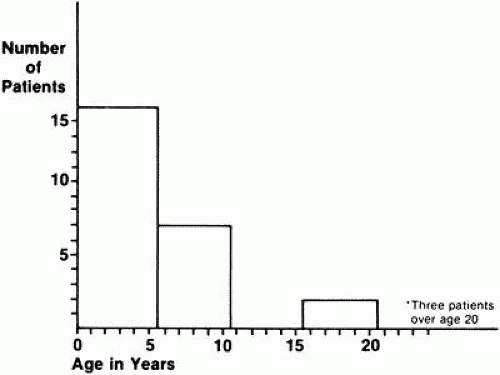 Fig. 1. Reported age at onset of night blindness for patients with type I simplex-multiplex retinitis pigmentosa. (Adapted from Massoff RW, Boughman JA: Genetic analysis of subgroups within simplex and multiplex retinitis pigmentosa. In Cotlier E, Maumenee IH, Berman ER [eds]: New York, Alan R. Liss for the March of Dimes Birth Defects Foundation, BD:OAS 18[6]: 161–166, 1982) |
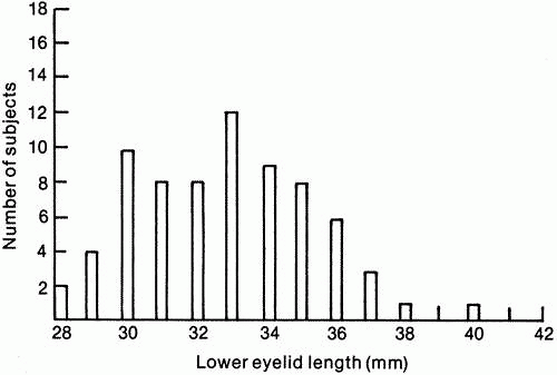 Fig. 2. Length of lower eyelid for women age 50 and older. (Data from Lin D, Strasior OG: Lower eyelid laxity and ocular symptoms. Published with permission from The American Journal of Ophthalmology 95:545–551, 1983. Copyright © by The Ophthalmic Publishing Company.) |
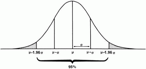 Fig. 3. Normal distribution showing mean (μ), standard deviation (σ). |
The importance of understanding the distribution of a particular set of data is twofold. Not only is it a way of taking a large collection of disorganized observations and condensing the information into a cohesive and understandable format, but recognizing the underlying distribution of the data is essential to choosing appropriate methods of analysis.
Once the general form of the distribution is decided on, we can proceed either to describe the data in more detail or to make inferences from what we see. In clinical ophthalmology, statistics is primarily used for inference. However, a simple example from descriptive statistics best illustrates the usefulness of parameters of a distribution. Because so many measurements of human beings are take a normal distribution, this distribution is sometimes assumed without specification in statements such as “the normal intraocular pressure is 15.5, with a standard deviation of 2.6.” Statistics provides a more exact mathematical way to say, “most people have IOPs of around 15.” In particular, it gives a precise definition of “around 15,” which can be important, for example, for interpreting an intraocular pressure of 18 (still in the middle part of the distribution) or 35 (in the far right tail of the distribution).
STANDARD DEVIATIONS AND STANDARD ERRORS
The standard deviation is a very simple concept. Figure 3 shows a normal curve with its mean and standard deviation. Notice that the line describing the normal curve is concave downward in the middle and concave upward toward each end. The point of inflection (point at which the curve reverses) is one standard deviation away from the mean (middle) of the curve. The standard deviation, usually denoted with a lower case sigma (σ), is a simple way of describing how “scattered out” the observations are. The standard deviation has other useful characteristics for Normally distributed variables. Approximately two thirds of the values lie within one standard deviation of the mean (in the example above, intraocular pressures between 12.9 and 18.1). Ninety-five percent of the values fall within approximately two standard deviations of the mean (1.96 standard deviations, to be exact). This means that there is a good mathematical reason to categorize as “high” a value that is more than two standard deviations above the mean. Only two and a half percent of individual values in a normal distribution are this far above the mean. Conversely, a value two standard deviations (or more) below the mean of a normal distribution can reasonably be defined as “significantly” low. In Figure 3, the shaded area represents all observations at least 1.96 standard deviations away from the mean in either direction. This is an important point to remember, because it is the basis for many statistical tests. Because the curve is symmetric, 2.5% of observations lie more than 1.96 standard deviations above the mean (“in the right tail”) and 2.5% are at least this distance below the mean, or in the left tail. The standard deviation of a distribution is denoted with a lower case sigma (σ). (Statisticians are also interested in the square of the standard deviation, called the variance of the distribution, but discussion of the latter statistic is beyond the scope of this chapter.)
INFERENCE
In ophthalmology, statistics is most commonly used to infer something about a population on the basis of observations made on a sample taken from that population. (Statisticians use the word “population” quite generally to refer to all the values in a distribution—intraocular pressures, outcomes of a treatment, and so on, not just individual human beings.) The intraocular pressures recorded for one ophthalmologist’s patients can be thought of as a sample (unfortunately, not a random sample) of the unknowable population intraocular pressures for all patients. In descriptive statistics, exact values are computed for parameters such as the mean and standard deviation, describing persons actually studied. In statistical inference, it is important to distinguish between the true (and usually unknown) value of a parameter in a population and the numeric estimate of that parameter based on measurements obtained from a sample of the population. The “true” value is generally denoted by a Greek letter, and numeric estimates by the English alphabet. Thus
, the sample mean or average, is an estimate of the true mean, μ, for the population and SD or s is used to denote an estimate of σ, the population standard deviation. A common way to represent results is to give the “mean ± 1 SD.” For example, the data in Figure 2 can be summarized by the statement “mean = 32.82 ± 2.54 mm.” It should be noted, however, that some authors use this same format to present the mean and the standard error of the mean. The latter statistic represents something quite different.
Stay updated, free articles. Join our Telegram channel

Full access? Get Clinical Tree


