Visual Fields in Glaucoma
Jody R. Piltz-Seymour
Tak Yee Tania Tai
Sanjay Smith
Stephen M. Drance
THE NORMAL VISUAL FIELD
The field of vision is defined as the area that is perceived simultaneously by a fixating eye. The limits of the normal field of vision are 60° into the superior field, 75° into the inferior field, 110° temporally, and 60° nasally (Fig. 49-1). Traquair,1 in his classic thesis, described an island of vision in a sea of darkness (Fig. 49-2). The island represents the perceived field of vision, and the sea of darkness is the surrounding area that is not seen. In the light-adapted state, the island of vision has a steep central peak that corresponds to the fovea, the area of greatest retinal sensitivity. From the peak, the island slopes downward toward the periphery, which represents regions of diminishing retinal sensitivity. The physiologic blind spot corresponds to the area of the optic nerve head. It is visualized as a deep well to sea level 15° temporal to the peak of the island.
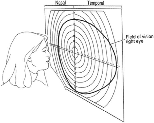 Figure 49-1. Limits of the normal visual field, right eye: 60° superiorly, 75° inferiorly, 110° temporally, and 60° nasally. |
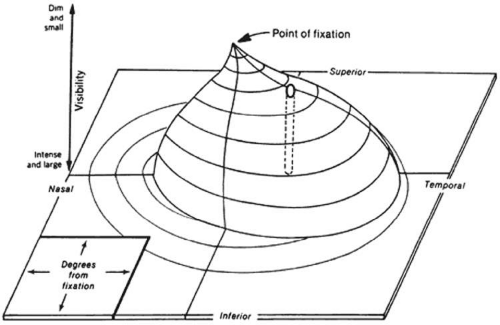 Figure 49-2. The normal island of vision. The hill is highest at fixation, where visual sensitivity is greatest. The height of the hill of vision declines toward the periphery as visual sensitivity diminishes. (Reproduced with permission from Anderson DR: Perimetry with and without Automation. 2nd ed. St Louis, MO: Mosby, 1987.) |
The contour of the island of vision relates to both the anatomy of the visual system and the level of retinal adaptation. The sharp-peaked island of vision described by Traquair reflects the visual field in the light-adapted or photopic visual field. The highest concentration of cones is in the fovea; most of these cones project to their own ganglion cell. This one-to-one ratio between foveal cone and ganglion cell results in maximal resolution in the fovea.
The contour of the island of vision changes greatly in the mesopic (twilight) and scotopic (dark-adapted) states. As one proceeds from a photopic to a scotopic state, overall retinal sensitivity increases as rod, rather than cone, vision predominates. In the dark-adapted island of vision, the contour is flatter than in the light-adapted state, and a central depression, rather than a central peak, exists in the area of the fovea. Thus, the level of retinal adaptation is crucial in defining the contour of the island of vision (Fig. 49-3).2
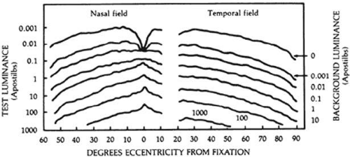 Figure 49-3. Aulhorn curves show the influence of background luminance on the differential light threshold. As the background luminance increases (lower curves) and the retina becomes light adapted (i.e., photopic adaptation), the overall retinal sensitivity decreases and the curve peaks centrally at the fovea. As the background luminance decreases (upper curves) and the eye becomes dark adapted (i.e., scotopic adaptation), overall retinal sensitivity increases and the curves develop a central depression. (Reproduced with permission from Lynn JR, Fellman RL, Starita RJ: Exploring the normal visual field. In Ritch R, Shields MD, Krupin T (eds): The Glaucomas, vol 1. St Louis, MO: Mosby, 1989.) |
METHODS OF MEASURING THE VISUAL FIELD
STATIC PERIMETRY
Manual static perimetry was introduced into clinical practice by Aulhorn and Harms on the basis of the research carried out by Sloane. It was the preferred method of examination in various European and North American centers and was the precursor of computerized perimetry. Most perimetry performed now is computerized static perimetry. One of the first computerized automated perimeters was developed in 1972 by Franz Fankhauser at the University of Berne and the first commercial unit was developed by Octopus in 1974.
In static perimetry, retinal sensitivity is measured at fixed locations by varying the brightness of the test target. The size of the target is kept constant. The shape of the island of vision is defined by repeating the threshold measurement at various locations in the field of vision (Fig. 49-4).
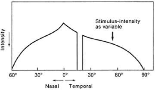 Figure 49-4. In static perimetry, the intensity of a stationary target of constant size is varied to determine the sensitivity of specific locations in the field of vision. |
KINETIC PERIMETRY
Kinetic perimetry is usually performed manually on the Goldmann perimeter or the tangent screen, although a few automated instruments offer kinetic modules. In kinetic perimetry, a stimulus is moved from a non-seeing area of the visual field to a seeing area along a set meridian. The procedure is repeated with the use of the same stimulus along other meridians, usually spaced every 15°. In kinetic perimetry, one attempts to find locations in the visual field of equal retinal sensitivity. By joining these areas of equal sensitivity, an isopter is defined. The luminance and the size of the target are changed to plot other isopters. In kinetic perimetry, the island of vision is approached horizontally. Isopters may be considered the outline of horizontal slices of the island of vision (Fig. 49-5).3
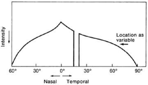 Figure 49-5. In kinetic perimetry, a stimulus of set size and intensity is moved from nonseeing to seeing areas of the visual field. The island of vision is approached horizontally, and isopters, depicting areas of equal retinal sensitivity, are plotted. |
STATIC COMPUTERIZED AUTOMATED PERIMETRY
Computers and automation permit static testing to be performed in an objective and standardized fashion, which minimizes perimetrist bias. A quantitative representation of the visual field can be obtained more rapidly than with manual testing. The computer presents stimuli in a pseudorandom, unpredictable fashion; patients do not know where the next stimulus will appear, improving fixation and increasing reliability of the test. Random presentations also increase the speed with which perimetry can be performed by bypassing the problem of local retinal adaptation, which requires a 2-second interval between stimuli if adjacent locations are tested.
Computerized static perimetry provides an estimate of the reliability and variability of the test. Data storage is possible, and computer-assisted statistical analysis is available.4
The most widely used automated perimeters are manufactured by Carl Zeiss Meditec Inc. (Humphrey Field Analyzer [HFA] and frequency-doubling technology [FDT]) and Haag -Streit International (Octopus). Other perimeters also provide comparable thresholding tests; testing strategies and statistical analyses vary between instruments. Most automated perimeters perform a wide variety of programs so that examinations can be tailored to the needs of individual patients.
DIFFERENTIAL LIGHT THRESHOLD
Static computerized perimetry measures retinal sensitivity at predetermined locations in the visual field. These perimeters measure the eye’s ability to detect a difference in contrast between a test target and the background luminance. Classically, threshold is defined as the dimmest target seen 50% of the time; however, different perimeters have varied strategies to efficiently measure the differential light threshold. These strategies are described later in this chapter under Automated Perimetry: Testing Strategies: Threshold Programs.
APOSTILBS AND DECIBELS
In perimetry, luminance of test targets is measured in apostilbs (asb). An apostilb is an absolute unit of luminance that is equal to 0.3183 candela/m2, or 0.1 millilambert.
The decibel scale is a relative scale created by the manufacturers of automated perimeters to measure the sensitivity of the island of vision. It is an inverted logarithmic scale. Zero decibels is set as the brightest stimulus that the perimeter can produce. The decibel scale is not standardized because the maximal luminance varies between instruments.
Table 49-1 shows the relationship between apostilbs and decibels for the Humphrey Field Analyzer (HFA) where zero decibels corresponds to 10,000 asb. A change of 10 dB equals a 1 log unit or tenfold change in intensity, and 1 dB is equivalent to 0.1 log unit.
Table 49-1. Apostilbs and Decibels on the Humphrey | ||||||||||||||
|---|---|---|---|---|---|---|---|---|---|---|---|---|---|---|
|
Does a threshold of zero mean that the patient is blind at that location? Not necessarily. It simply means that the patient was not able to distinguish the brightest spot that the machine projected from the background luminance.
SENSITIVITY VERSUS THRESHOLD
As one ascends the hill of vision toward the fovea, the sensitivity of the retina increases, dimmer targets become visible, and the brightness of the target at threshold decreases. Therefore, as retinal sensitivity increases, the differential light threshold measured in apostilbs decreases. This inverse relationship between retinal sensitivity and threshold holds true throughout most of visual psychophysics. In automated perimetry, however, threshold is recorded in the inverted decibel scale, and dimmer targets have higher decibel values. Therefore, threshold in decibels is directly proportional to retinal sensitivity.
MANUAL PERIMETRY: THE VISUAL FIELD ON THE GOLDMANN PERIMETER
In 1945 Hans Goldmann introduced a manual perimeter that standardized the manual visual field testing process. For decades, the Goldmann perimeter was the most widely used apparatus for visual field testing. It is a calibrated bowl projection instrument with a background intensity of 31.5 asb, which is well within the photopic range. The size and intensity of targets may be varied to plot different isopters kinetically and determine local static thresholds.5
The stimuli used to plot an isopter are identified by a Roman numeral, a number, and a letter. The Roman numeral represents the size of the object, from Goldmann size 0 (1/16 mm2) to Goldmann size V (64 mm2) (Table 49-2). Each size increment equals a twofold increase in diameter and a fourfold increase in area.
Table 49-2. Size of Goldmann Targets | |||||||||||||||||||||
|---|---|---|---|---|---|---|---|---|---|---|---|---|---|---|---|---|---|---|---|---|---|
|
The number and letter represent the intensity of the stimulus. A change of one number represents a 5 dB (0.5 log unit) change in intensity, and each letter represents a 1 dB (0.1 log unit) change in intensity (Table 49-3). The dynamic range of the Goldmann perimeter from the smallest/dimmest target (Ola) to the largest/brightest target (V4e) is >4 log units, or a 10,000-fold change.
Table 49-3. Intensity of Goldmann Targets | ||||||||||
|---|---|---|---|---|---|---|---|---|---|---|
|
More than 100 combinations of size and intensity are available, but only a few isopters are needed to define the visual field. Size 0 generally is omitted because results of the plots are inconsistent. The fine-intensity filter is usually set to the letter e, which eliminates the small-increment light filters.
A change of one number of intensity is roughly equivalent to a change of one Roman numeral of size. Isopters in which the sum of the Roman numeral (size) and number (intensity) are equal can be considered equivalent. For example, the I4e isopter is roughly equivalent to the II3e isopter. The equivalent isopter combination with the smaller size 1 target is usually preferred because detection of isopter edges is more accurate with smaller targets. One usually starts by plotting small targets with dim intensity (I1e) and then increasing the intensity of the target until it is maximal before increasing the size of the target. The usual progression then is I1e→I2e→I3e→I4e→II4e→III4e→IV4e→V4e (Fig. 49-6).
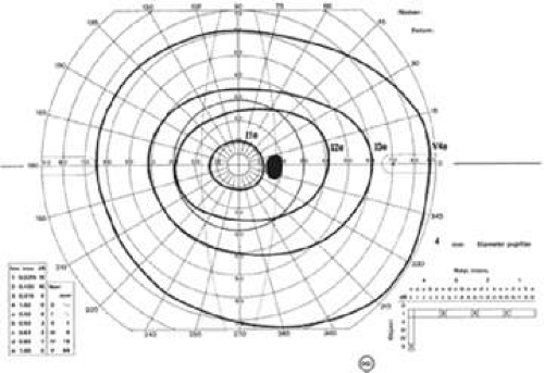 Figure 49-6. Standard isopters on the Goldmann perimeter for the right eye of a normal 43-year-old patient. The Roman numeral identifies the stimulus size, and the arabic numeral and letter identify the stimulus intensity. |
In addition to plotting isopters kinetically, static suprathreshold and threshold testing can be performed manually. After an isopter has been plotted, the stimulus used to plot the isopter is used to test statically within the isopter to look for localized defects. In this way, it acts as a suprathreshold stimulus. Static thresholds also can be determined along set meridians to obtain profile plots of the visual field, but like any multiple thresholding task, it is time consuming.
Manual kinetic perimetry allows fast, flexible, comprehensive evaluation of the entire visual field. However, shallow scotomas can be missed and isopters may be hard to define if the slope of the island of vision is not steep (Fig. 49-7). The quality of the field test is highly dependent on the skill of the perimetrist. Results from different perimetrists can vary greatly.
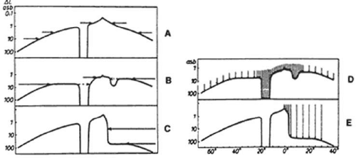 Figure 49-7. Comparison of static and kinetic perimetry to detect shallow scotomas and determine the slope of the scotoma. A. Kinetic evaluation can clearly outline the normal visual field. B. Kinetic perimetry may miss shallow scotomas and poorly define the flat slope seen nasally. C. The edge of steeply sloped scotomas may be identified easily with kinetic perimetry, but the steepness of the slope may not be appreciated. D and E. Static perimetry readily detects shallow scotomas and can define the slope of both shallow and steep scotomas. (Reproduced with permission from Aulhorn E, Harms H: Early visual field defects in glaucoma. In Leydecker W (ed): Glaucoma Symposium. Basel, Germany: Karger, 1966.) |
GLAUCOMATOUS VISUAL FIELD DEFECTS
Any clinically or statistically significant deviation from the normal shape of the hill of vision can be considered a visual field defect. The classic glaucomatous defect is a localized scotoma that conforms to nerve fiber bundle patterns. Diffuse depressions of the visual field are also commonly seen in glaucomatous eyes but are often difficult to distinguish from nonglaucomatous causes of such diffuse depressions of the visual field.
LOCALIZED NERVE FIBER BUNDLE DEFECTS
Localized visual field defects in glaucoma result from damage to the retinal nerve fiber bundles. Because of the unique anatomy of the retinal nerve fiber layer, axonal damage causes characteristic patterns of visual field damage.
Anatomy of the Nerve Fiber Layer
The nerve fiber layer of the retina is composed of ganglion cell axons that course from the ganglion cell body to the optic nerve head in a distinctive pattern (Fig. 49-8). The optic nerve lies 15° nasal and slightly superior to the fovea. The retina temporal to the fovea is divided into superior and inferior halves by the horizontal raphe. Axons that originate in the superior half of the temporal retina arch above the fovea, whereas those that originate inferior to the raphe arch below the fovea. These arching temporal fibers form the arcuate nerve fiber bundles and enter the optic nerve head at the superior and inferior poles.6
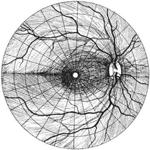 Figure 49-8. The retinal nerve fiber layer in the right eye. Damage to localized bundles of nerve fibers results in characteristic patterns of visual field loss in glaucoma. (Reproduced with permission from Harrington DO, Drake MV: The Visual Fields: Textbook and Atlas of Clinical Perimetry. St Louis, MO: Mosby, 1990.) |
The papillomacular fibers from the central retina and the fibers from the nasal retina course directly from their cell bodies to the disc.
Nerve Fiber Bundle Defects
The superior and inferior poles of the optic nerve head are most vulnerable to glaucomatous damage. It has been postulated that these areas may be watershed areas at the junction of the vascular supply from adjacent ciliary vessels.7 Ultrastructural examination of the lamina cribrosa shows that the pores in the superotemporal and inferotemporal areas are larger. These larger pores may make these regions more vulnerable to compression.8
Damage to the inferior and superior poles of the nerve results in loss of the arcuate nerve fiber bundles. The resulting visual field defect types include paracentral, arcuate, and nasal step. The inferior pole of the optic nerve appears to be more vulnerable to damage than the superior poles, so that defects occur more commonly in the superior half of the visual field.
PARACENTRAL DEFECTS
Circumscribed paracentral defects are an early sign of localized glaucomatous damage. These defects may be absolute when first discovered, or they may have deep nuclei surrounded by areas of less dense involvement. The dense nuclei often are numerous along the course of the nerve fiber bundle (Fig. 49-9). A relative disturbance often can be traced between a dense paracentral scotoma and the blind spot; it may vary in extent, but it shows the true arcuate nature of the scotoma. Paracentral defects often lie closer to fixation when they occur in the superior hemifield.
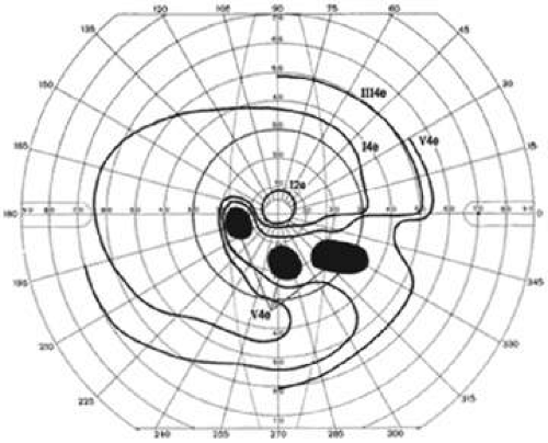 Figure 49-9. Multiple dense paracentral defects in an arcuate nerve fiber bundle distribution. |
ARCUATE SCOTOMAS
More advanced loss of arcuate nerve fibers leads to a scotoma that starts at or near the blind spot, arches around the point of fixation, and terminates abruptly at the nasal horizontal meridian (Fig. 49-10). An arcuate scotoma may be relative or absolute. In the temporal portion of the field, it is narrow because all of the nerve fiber bundles converge onto the optic nerve. The scotoma spreads out on the nasal side and may be very wide along the horizontal meridian. Arcuate scotomas may develop closer to fixation in myopic patients.
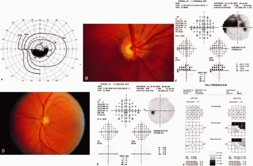 Figure 49-10. Arcuate and nasal step defects. A. Goldmann kinetic perimetry. B. Right optic nerve with inferior notch. C. The corresponding full threshold visual field of the right eye with superior defect. D. Left optic nerve of the same patient with intact neural rim with inferior disc hemorrhage and early nerve fiber layer defect. E. The corresponding full threshold field did not pick up the early defect in the left eye. F. Frequency doubling technology field testing. Superior defect detected in the right eye. The early nerve fiber layer defect was not detected in the left eye. |
NASAL STEP DEFECTS
Because of the anatomy of the horizontal raphe, all complete arcuate scotomas end at the nasal horizontal meridian. A steplike defect along the horizontal meridian results from asymmetric loss of nerve fiber bundles in the superior and inferior hemifields.
In manual perimetry, nasal step defects may be evident in some isopters but not in others, depending on which nerve fiber bundles have been damaged. The width of the nasal step also varies. Nasal steps frequently occur in association with arcuate and paracentral scotomas, but a nasal step may also occur in isolation. The earliest initial visual field defects in approximately 7% of glaucoma patients are nasal step defects outside of the central 30°, which may be missed by routine automated perimetry programs.
TEMPORAL WEDGE-SHAPED DEFECTS
Damage to nerve fibers on the nasal side of the optic disc may result in temporal wedge-shaped defects (Fig. 49-11). These defects are much less common than defects in the arcuate distribution. Occasionally, they are seen as the sole visual field defect. Temporal wedge defects do not respect the horizontal meridian. They frequently occur in myopic patients.
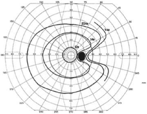 Figure 49-11. Temporal wedge defect. |
EARLY VISUAL FIELD DEFECTS
The appearance of a discrete, localized visual field defect may be preceded by inconsistent or fluctuating responses in that area.9,10 Initial localized visual field defects may be either relative or absolute. In 35 eyes with previously normal visual fields, Werner and Drance10 found that the earliest defects were paracentral scotomas with a nasal step (51%), isolated paracentral defects (26%), isolated nasal steps (20%), and sector defects (3%). Hart and Becker11 found the following initial visual field defects in 98 eyes: nasal steps (54%), paracentral or arcuate scotomas (41%), arcuate blind spot enlargement (30%), isolated arcuate scotomas separated from the blind spot (20%), and temporal defects (3%).
Phelps et al12 reported the location of localized visual field defects in eyes with chronic open-angle glaucoma whose maximum intraocular pressure ranged from 22 to 34 mm Hg (Fig. 49-12). The superior field was involved more often than the inferior visual field, and the nasal periphery frequently was affected.
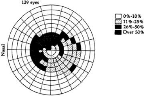 Figure 49-12. Frequency distribution of visual field defects in eyes with chronic open-angle glaucoma. Maximum intraocular pressures ranged between 22 and 34 mm Hg. (Reproduced with permission from Lynn JR, Fellman RL, Starita RJ: Exploring the normal visual field. In Ritch R, Shields MD, Krupin T (eds): The Glaucomas, vol 1. St Louis, Mo: Mosby, 1989.) |
BLIND SPOT CHANGES
Enlargement
Vertical elongation of the blind spot to a suprathreshold stimulus leads to the development of a Seidel scotoma, an early arcuate defect that connects with the blind spot. β-Peripapillary atrophy, which frequently accompanies glaucomatous damage, particularly in elderly patients, also may cause an overall enlargement of the blind spot.
Baring
Physiologic baring of the blind spot is an artifact of kinetic perimetry. Because the inferior retina is less sensitive than the superior retina in most normal people, using a stimulus that is at threshold in the visual field just below the blind spot results almost always in a baring of the blind spot superiorly This physiologic baring of the blind spot is confined to the isopter plotted with such a threshold target (Fig. 49-13).
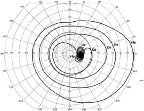 Figure 49-13. Physiologic superior baring of the blind spot usually is limited to a single central isopter. |
END STAGE DEFECTS
In eyes with advanced glaucomatous damage, arcuate fibers are lost, leaving only papillomacular and nasal fibers. The typical visual field in advanced glaucoma shows preservation of a small central island of vision and a larger temporal island of vision (Fig. 49-14). The temporal island of vision is not detected with most standard automated perimetry programs since temporal islands lie outside of the central 24 to 30°°.
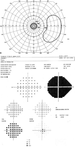 Figure 49-14. A. A visual field exhibiting end stage defects. Only a small central island and a temporal island of vision remain. B. End stage visual field defect on 24-2. In this figure, the pattern deviation plot appears abnormal. However, advanced defects may cause the pattern deviation plot not to appear grossly abnormal. This artifact occurs when there are fewer than eight points with measurable thresholds and is the result of the statistical processing of the pattern deviation plots. |
DIFFUSE DEPRESSION
Diffuse depression of the visual field results from an overall or widespread sinking of the island of vision and may reflect diffuse loss of nerve fibers of the retina. Diffuse depression is a nonspecific sign that can be caused by many entities other than glaucoma. By far the most common reason for a diffuse depression is lens opacity. Other factors include other media opacities, miosis, improper refraction, ocular anomalies, age, and patient fatigue, inattentiveness, or inexperience with the examination. It is therefore difficult to attribute diffuse depression specifically to a glaucomatous process unless the visual acuity is normal and the other causes of such depression can be excluded.
Hart and Becker11 found that of eyes that had localized visual field defects, 31% had constriction of the central isopters. Piltz et al13 used automated perimetry and found that approximately 50% of eyes with localized visual field defects had generalized depression in the absence of lens opacity. They noted that it was rare to identify purely diffuse glaucomatous visual field loss in the absence of localized defects. Of 91 patients with chronic open-angle glaucoma, only two had purely diffuse visual field loss.13 Diffuse depression of the visual field is not commonly seen as the only sign of glaucoma, but diffuse loss often occurs in conjunction with localized visual field defects.
In manual perimetry, diffuse depression is manifested by contraction of the isopters. The isopters retain their normal contour. The most central isopters may disappear entirely as the peak of the island of vision sinks (Fig. 49-15).
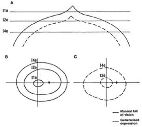 Figure 49-15. Diffuse visual field depression: manual kinetic perimetry. A. Profile plot showing a normal and depressed hill of vision. B. Isopter plot of the normal hill of vision. C. Isopter plot of a depressed hill of vision. Note the loss of the Ile isopter and the inward shifting of the I2e and I4e isopters in the field with generalized depression. |
In automated perimetry, diffuse depression results in relative defects across the entire visual field (Fig. 49-16). Early diffuse depression often is difficult to detect because thresholds may remain within the normal range, but they may be depressed from previous examinations or the baseline status. The deviation plots and probability maps help evaluate the influence of generalized depression. The total deviation plots include both localized and diffuse loss. For the pattern deviation plots, the diffuse loss is statistically removed, highlighting the localized loss. This is discussed further under Probability Plots.
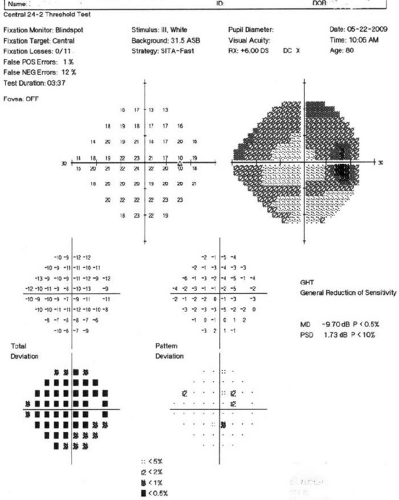 Figure 49-16. Diffuse visual field depression: automated perimetry. Mild relative defects are seen across the visual field. Many probability symbols are seen in the total deviation map, and few probability symbols are seen in the pattern deviation map. The glaucoma hemifield test reports a generalized reduction in sensitivity. The mean deviation is flagged as significantly abnormal, and the corrected pattern standard deviation is within normal limits. |
Cumulative defect curves (Bebie curves), found on the Octopus printouts, greatly facilitate the identification of diffuse visual field loss (Fig. 49-17). At each location in the visual field, the measured threshold is subtracted from the expected normal threshold for that point. This value is called the defect. The Bebie curve is simply a graphic ranking of the defects from least to greatest defect. The Bebie curve for a given patient can be interpreted in light of the confidence intervals plotted.14
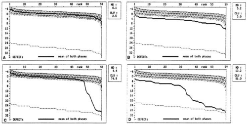 Figure 49-17. Bebie curves. Bebie, or cumulative defect, curves are useful in detecting diffuse depression of the visual field. The curve is a graphic ranking of the defect (the difference between the measured threshold and the age-corrected normal threshold) for each point in the visual field. The x axis represents the rank of the defect from smallest (left side) to largest (right side). The y axis represents the magnitude of the defect. The normal range, between the 5th and 95th percentiles, is shaded. A. A normal Bebie curve. The curve lies completely within the normal shaded area. B. The Bebie curve of a patient with diffuse damage. The Bebie curve is shifted inferiorly but parallels the normal range. C. The Bebie curve of a patient with purely localized damage. Most of the curve falls within the normal range; however, a sharp decline is measurable at the higher ranks. D. An example of combined localized and diffuse damage. The entire curve is depressed below normal range. The left side parallels the normal range and represents the diffuse loss. The decline on the right side represents the superimposed localized damage. (Courtesy of Balwantray C. Chauhan, PhD.). |
If the Bebie curve is evenly depressed below the 95th percentile, depression of the visual field is generalized. If only the right side of the curve is depressed, visual field loss is localized. If the whole curve is depressed but in an uneven fashion, both localized and diffuse loss is present. Although they are useful in identifying the type of visual field loss present, Bebie curves cannot distinguish between glaucomatous and nonglaucomatous causes of localized or diffuse visual field loss.
HOW DO VISUAL FIELD DEFECTS PROGRESS?
Despite control of intraocular pressure, many eyes with glaucoma exhibit progression of visual field defects over time. Most eyes exhibit an increase in the density of the scotoma, and approximately 50% exhibit an increase in scotoma size or the appearance of a new scotoma.15 Progression of defects may occur in episodic bursts intermixed with stable periods of varying duration. If only one hemifield is involved, the defects remain localized to that hemifield for extended periods in 60% to 75% of eyes. Progression often occurs more rapidly when both hemifields are involved.12 The mean level of intraocular pressure does not differentiate glaucoma patients with progressive visual field loss from those who remained stable.16
Prior rate of progression can help predict future risk of progression, and the risk of progression increases as visual field loss becomes more advanced. However, not all treated patients with end stage visual field loss progress to blindness. Much et al17 performed a retrospective review of 84 eyes of 64 patients with <10° islands of vision who were followed for an average of 100.1 ± 36.6 months; the vast majority of these patients with advanced loss maintained vision of 20/40 or better, and only 9.5% of patients progressed to a visual acuity of 20/200 or worse.
One study found that the average rate of visual field decline over a mean of 15.2 years of follow-up was – 1.3% per year. The rates (in percent per year) of visual field change by section from greatest to least were superonasal (-1.8), superior (-1.5), nasal (-1.4), peripheral (-1.4), central (-1.3), inferotemporal (-1.3), inferior (-1.2), inferonasal (-1.2), temporal (-1.2), and superotemporal (-1.1). Half the patients showed symmetric visual field decline. The presence of disc hemorrhage was found to be associated with asymmetric visual field progression.18
Stay updated, free articles. Join our Telegram channel

Full access? Get Clinical Tree


