and Donald T. Miller3
(1)
Vision Science and Advanced Retinal Imaging Laboratory (VSRI) Department of Ophthalmology and Vision Science, University of California Davis, 4860 Y Street, Ste. 2400 , Sacramento, CA 95817, USA
(2)
UC Davis RISE Eye–Pod Laboratory, Department of Cell Biology and Human Anatomy, University of California Davis, 4320 Tupper Hall, Davis, CA 95616, USA
(3)
School of Optometry, Indiana University, 800 East Atwater Avenue, Bloomington, IN 47405, USA
Keywords
Adaptive opticsAge-related macular degenerationChoroidal vasculatureColor blindness phenotypingEyeGlaucoma Image quality of the eyeImage registrationMacular TelangiectasiaMedical optics instrumentationMicroscopyMonochromatic and chromatic aberrationsMotion artifact correctionNon-invasive assessment of the visual systemOcular aberrationsOphthalmic opticsOphthalmologyOptic nerve headOptic neuropathiesOptical biopsyOptical coherence tomographyPhase-sensitive AO-OCTPhotoreceptorsPolarization-sensitive AO-OCTRetinaRetinal nerve fiber layerRetinal pigment epitheliumRetinal vasculatureRetinitis pigmentosaRetinopathy of prematurityWavefront correctorWavefront sensor61.1 Introduction
The last 20 years have experienced extraordinary advances in optical technology to image noninvasively and at high resolution the posterior segment of the eye. Two of the most impactful technological advancements over this period have arguably been optical coherence tomography (OCT) and adaptive optics (AO). OCT provides unprecedented, micron-scale axial resolution (<3 μm) and sensitivity to detect reflections from essentially any retinal layer, including those that are highly transparent [1, 2]. OCT has become a standard diagnostic tool for evaluating health of the posterior segment, for example, for macular holes, central serous chorioretinopathy, age-related macular degeneration, macular edema, diabetic retinopathy, and glaucoma.
Unlike OCT, AO is not an imaging modality, but rather a technology that can be used in combination with imaging modalities to improve their performance. AO works by measuring and correcting ocular aberrations at real time. Its benefit is greatest when the pupil is large (>6 mm), which has the added benefit of minimizing the blurring effects caused by diffraction. Correction of ocular imperfections across a large pupil results in unprecedented lateral resolution (2–3 μm), sufficient for resolving individual cells en face [3–5]. AO was originally developed for ground-based telescopes to remove atmospheric blur and later incorporated into retinal imaging in the mid-1990s. Since then, AO for the eye has experienced exponential growth resulting in the first textbook devoted to the topic in 2006 [4]. Essentially all facets of AO have undergone substantive development for use with the eye, including its wavefront sensor, wavefront corrector, and control algorithm. In addition, AO has been integrated into a wide range of retina camera architectures to increase their resolution and sensitivity including the three principle types: flood-illuminated ophthalmoscope [3, 6–9], scanning laser ophthalmoscope (SLO) [10–15], and OCT [16–28]. Collectively these have become a valuable suite of imaging tools for vision and clinical research. Individually, each has distinct technical strengths that define the types of fundus imaging applications they are best suited for.
The aim of this chapter is to focus on the latter combination: adaptive optics – optical coherence tomography (AO-OCT). Success of the individual technologies, AO and OCT, has led to considerable effort by several research groups over the last decade to combine them for high-resolution, three-dimensional imaging of the retina. The resulting 3D resolution holds considerable promise to improve the research and clinical utility of OCT: for probing structure and function of the microscopic retina and for earlier detection, more precise diagnosis, and improved treatment monitoring of posterior segment disease.
Several excellent chapters in this book already cover the theoretical and experimental underpinnings of OCT. Thus this chapter focuses on the other key aspects of AO-OCT, especially those important for the design and implementation of AO in OCT systems. With that overriding principle, the chapter is divided into three main parts. First is a summary of our current understanding of the key optical properties of the eye. These properties underlie the motivation for AO-OCT and define the design requirements of AO-OCT systems. This is followed by a discussion of AO technologies and the technical benefits of adding AO to OCT. The second part surveys AO-OCT designs reported in the literature. Unlike flood illumination and SLO modalities that have effectively one principle design configuration, OCT embodies several fundamentally different ones, resulting in a wide variety of AO-OCT systems that have been attempted. The last part reviews some of the latest scientific and clinical uses of this powerful technology and a look to future developments in this rapidly growing field.
61.2 Imaging Properties of the Eye
The eye is unique, unlike any other organ in the body, it represents a complete imaging system including refracting optics (cornea and crystalline lens), aperture (iris), and photosensitive detector (retina/fundus). All of these are of course necessary for the eye to perform its critical function, vision, which it does amazingly well. However, when we purposely reverse the direction of light to view the retina and fundus, for example, examination with OCT, the completeness of the system – in particular the ocular media and iris – is less than ideal. The ocular system imposes severe constraints on how well we can image the back of the eye and the finest microscopic detail we can resolve.
Improved understanding of the optical properties of the eye has enabled AO-OCT to surpass the natural lateral resolution limits imposed by our eyes. This required overcoming the eye’s intrinsic monochromatic and chromatic aberrations and minimizing its diffraction effects. Here we summarize the pertinent aspects of each for AO-OCT imaging. Our discussion is limited to the human eye, but it is worth noting that there is growing activity in experimental imaging in animal models using the same technology [29, 30].
61.2.1 Monochromatic Aberrations of the Eye
Monochromatic aberrations of the eye vary spatially across the eye’s pupil, vary over time, and vary with field location at the retina. These fundamental properties (spatial, temporal, and field dependence) dictate the performance requirements of AO for effective correction of ocular aberrations and are discussed in order below.
The spatial distribution of ocular aberrations varies considerably among subjects and often does not correspond to the classical aberrations of manufactured optical systems, for example, Seidel aberrations. Instead, Zernike polynomials – orthonormal over circular pupils – are the most popular for representing ocular aberrations [31, 32]. Zernikes are not the most efficient polynomial representation of the eye’s aberrations, but are only slightly less compact than the principal modes that derive from a principal components analysis [33, 34]. Zernikes are also mathematically simpler and have well-established properties. The now ubiquitous use of Zernike polynomials is perhaps best reflected by the vision community’s establishment and universal acceptance of a single naming convention for the Zernike coefficients and polynomials as described by the OSA/VSIA Standards Taskforce [35].
Today monochromatic aberrations of the eye are well characterized. Detailed measurements of the spatial distribution of wave aberrations for central vision have been made in large populations of normal, healthy adult eyes with large pupils [33, 34, 36], including the pooling of data collected at ten laboratories (2,560 eyes) [37]. More recent studies have also been reported, including a retrospective analysis of 24,000 patients [38], expansion to peripheral aberrations [39, 40], and the effects of age, accommodation, refractive state, refractive surgery, and disease [41–49].
The spatial characteristics of the ocular aberrations most important for AO are spatial fidelity (frequency composition) and magnitude (peak-to-valley (PV) wavefront error). Both are captured by the Zernike representation – spatial fidelity by the Zernike order and magnitude by the Zernike coefficient – and both are strongly influenced by pupil size. As an example, Fig. 61.1 (left) shows the wavefront variance decomposed by Zernike order for a population of about 100 normal subjects, most in their early twenties [34]. Data points are shown for three pupil sizes, 4.5, 6.0, and 7.5 mm, which span the range over which AO is typically applied to the human eye. For comparison, the maximum physiological pupil size for young subjects is nominally 8 mm. In Fig. 61.1 (left), the power decreases monotonically (approximately linear on a logarithmic scale) with second-order aberrations dominating the total wavefront error. Power also decreases monotonically with decreasing pupil size. The 7.5 mm pupil represents the most demanding condition for AO and requires correction of Zernike polynomials up through at least tenth order to reach diffraction-limited imaging.
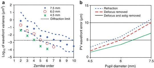
Fig. 61.1
Spatial properties of ocular aberrations in a large population of 100 normal eyes. (a) Log 10 of the wavefront variance after a conventional refraction using trial lenses is plotted as a function of Zernike order and pupil size (4.5, 6.0, and 7.5 mm). Diamonds and corresponding dashed curves represent the mean and mean ± two times the standard deviation of the log10(wavefront variance), respectively, for a 7.5 mm pupil. Star and open circle correspond to 4.5 and 6.0 mm pupils. Thin, horizontal dashed line corresponds to λ/14 RMS for λ = 0.6 μm. (b) PV wavefront error that encompasses 95 % of the population is plotted as a function of pupil diameter. Three second-order states are shown: (i) residual aberrations after a conventional refraction using trial lenses (short dashed lines), (ii) all aberrations present with zeroed Zernike defocus (long dashed lines), and (iii) all aberrations present with zeroed defocus and astigmatism (solid lines) (Reproduced with permission from OSA, Ref. [5])
Figure 61.1 (right) shows the corresponding PV wavefront error that encompasses 95 % of the population as a function of pupil size (4.5–7.5 mm). Three curves are shown that correspond to three different second-order states (defined in the figure caption). As expected, the PV error increases monotonically with pupil size and is strongly dependent on the second-order state. The PV error for the 7.5 mm pupil ranges from 7 to 11 μm depending on the second-order state. The largest error of 11 μm represents the most demanding condition for AO correction. Note that for this study, each subject was meticulously refracted with trial lenses. Typically, AO systems operate under less ideal conditions in which the second-order aberrations are only coarsely corrected or not at all. Under these non-ideal conditions, second-order aberrations can readily surpass the PV error shown in the figure by several times. As such, careful design of an AO system must take into account the anticipated refractive state of the population and the expected manner in which corrective trial and translating lenses and other means are applied in conjunction with AO.
Figure 61.2 provides a sense of the refractive state across eyes, showing cross-sectional refractive error distributions from several studies [50]. The distribution is not simple. It depends on many factors including population, age, education, and refractive state. Based on the figure distributions, a reasonable design goal for AO might be to correct errors up to +/−5 diopters as that covers a large percentage of eyes regardless of the factors shown.
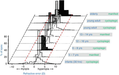
Fig. 61.2
Refractive error distributions sorted by age group and refraction (manifest or cycloplegic) (Graph reproduced and modified with permission from Elsevier, Ref. [50])
The population measurements in Fig. 61.1 represent essentially static wave aberrations and therefore do not capture the temporal behavior of the ocular media. Two early pivotal studies elucidated the temporal dynamics using a power spectral method and investigated their impact on AO performance [51, 52]. Figure 61.3 (left) shows results from one of these studies, specifically temporal traces of the wavefront error for one subject and a model eye and (right) the corresponding temporal power spectra. As suggested in the figure, temporal fluctuations are found in all of the eye’s aberrations, not just defocus, even when the eye’s accommodation is paralyzed. In both studies, the reported temporal fluctuations decreased at f −4/3, where f is the temporal frequency. This decrease is evident in the temporal power spectrum shown in Fig. 61.3 (right). The vast majority of the aberration power lies below 1–2 Hz, suggesting effective AO correction needs only a temporal bandwidth of a couple Hertz and an AO loop rate roughly 20 times faster.
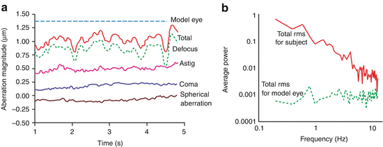
Fig. 61.3
Temporal properties of ocular aberrations [51]. (a) Temporal traces of the total RMS wavefront error and Zernike terms: defocus, astigmatism, coma, and spherical aberration for one subject. A trace of the total RMS wavefront error for an artificial eye is also shown and reflects the sensitivity of the instrument. (b) Average temporal power spectra are shown for the fluctuations in the total RMS wavefront error for a model eye and one subject whose accommodation was paralyzed. Aberrations were computed for a 4.7 mm pupil size (Reproduced with permission from OSA, Ref. [51])
Finally monochromatic aberrations of the eye also vary with field location at the retina. That is, image quality (or more precisely the point spread function or optical transfer function) at one point on the retina differs from that at another point when sufficiently separated. This difference in image quality stems from the fact that the ocular aberrations originate at the cornea and crystalline lens rather than at the pupil of the eye. Rays originating from different field locations on the retina will therefore take slightly different paths through the ocular media, accumulating different phase delays or equivalently different aberrations. In general there is a local region about any point on the retina in which the path differences are sufficiently small that the ocular aberrations are effectively constant. This region is termed the isoplanatic patch [53]. The diameter of the patch depends on the properties of the eye, but also on the definition of image quality, for example, use of the stringent Maréchal criterion, λ/14 μm RMS (Strehl ratio = 0.8) yields a narrower isoplanatic diameter than the more relaxed criterion of 1 rad2 (Strehl ratio = 0.37).
Anecdotal evidence in the AO literature indicates the isoplanatic patch diameter for the human eye is a couple of degrees. Experiments to directly measure the patch size have only recently been conducted. A detailed survey of efforts in this area coupled with a more thorough analysis was published by Bedggood et al. [54]. Figure 61.4 shows a representative result from this study, plotting isoplanatic patch diameter as a function of the residual wavefront RMS at the patch edge. As expected, the patch size increases as the criterion relaxes, i.e., larger residual RMS. As an example, diffraction-limited AO-OCT imaging at 850 nm wavelength requires a wavefront RMS correction of 61 nm or better. Using this as a criterion for the residual RMS at the patch edge in Fig. 61.4, the corresponding isoplanatic diameter is predicted to be somewhat less than one degree consistent with anecdotal evidence and other measurements reported in the literature. The narrowness of the isoplanatic patch has severe clinical consequences for AO-OCT as images at the isoplanatic size are substantially smaller than those collected with standard clinical instruments, a point illustrated by Fig. 61.3 (right). Shown is a fundus photograph with a standard 45° field of view and a 1° isoplanatic patch superimposed. While the fundus photograph can be captured in a single flash, AO-OCT performing at the diffraction limit requires tiling of 2,000 1° images – each with its unique AO correction – to cover the same field!
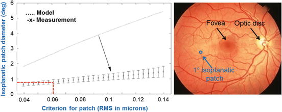
Fig. 61.4
(left) Isoplanatic properties of ocular aberrations. Isoplanatic patch diameter is plotted versus residual wavefront RMS at the patch edge after perfect correction of ocular aberrations at the patch center. Data points are average measurements across seven healthy subjects with error bars at ±1 standard deviation. Predicted patch diameter is also shown using the Liou Brennan schematic eye that clearly overestimates the measured diameter by several times [55]. Pupil size for both is 6 mm (Reproduced with permission from SPIE, Ref. [54]). (right) A 1° isoplanatic patch is superimposed on a conventional 45° fundus image, illustrating the vast difference in size
61.2.2 Chromatic Aberrations of the Eye
In addition to monochromatic aberrations, the human eye also suffers from significant chromatic ones (see Fig. 61.5), due primarily to its watery composition whose refractive index varies with wavelength. The longitudinal (LCA) and transverse (TCA) components of the ocular chromatic aberrations have been extensively studied at visible [56] and more recently near-infrared wavelengths up to 1,070 nm [57–59]. LCA and TCA refer to the variation in focus and image size with wavelength, respectively, both effectively blurring the patient’s vision or conversely the retinal image. Historically, interest in chromatic aberrations of the eye was driven by their impact on visual performance. This led to the design of numerous achromatizing lenses [60–65], many of which were shown effective at correcting the eye’s LCA, which is largely uniform across eyes and insensitive to field angle.
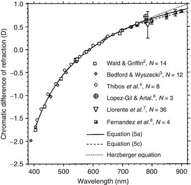
Fig. 61.5
Chromatic difference of refraction from several experimental studies and theoretical models that collective cover the visible spectrum and extend into the near infrared. All data were set to be zero at 590 nm. Close agreement between studies occurs largely because of the relatively small intersubject variation in chromatic aberrations [58]. (Reproduced with permission from OSA, Ref. [58])
In contrast, correcting the eye’s TCA has proven significantly more difficult, partly as TCA varies across eyes and is highly sensitive to field angle. In some cases, slight misalignment of the achromatizing lens to the eye was found to substantially increase the TCA, well above that which is intrinsic to the eye. Despite the mixed success of using achromatizing lenses to improve visual performance, its recent use in high-resolution retinal imaging, in particular AO-OCT, has proven beneficial. AO-OCT instruments have several key attributes that reduce the demand on the achromatizing lens. These include a comparatively small field of view, imaging at near-infrared wavelengths, a limiting pupil that is specified by the retina camera rather than the eye, better stabilization of the subject’s head, and raster scanning of the retina using galvanometer scanning mirrors.
61.2.3 Image Quality of the Eye
Retinal image quality is degraded not only by aberrations, but also diffraction, which for pupil diameters of less than about 3 mm is actually the largest source of image blur. A pupil about 3 mm in diameter – which is a typical pupil size under bright viewing conditions – generally provides the best optical performance in the range of spatial frequencies that are important for normal vision. Increasing the pupil size does increase the high-spatial-frequency cutoff, allowing finer details to be discerned, but at the high cost of increasing the deleterious effects of aberrations. Clearly, the very best optical performance would come from correcting all the eye’s aberrations across the dilated pupil.
Quantitatively, the effects of diffraction and aberrations on corrected and uncorrected pupils of various diameters are best illustrated by the modulation transfer function (MTF). Figure 61.6 shows the MTF for normal pupils 3 and 7.3 mm in diameter and for a large corrected 8 mm pupil. The large corrected pupil has a higher optical cutoff frequency and an increase in contrast across all spatial frequencies. Peering inward through normal-sized pupils, only large cell bodies (ganglion and retinal pigment epithelium) and the largest cone photoreceptors and capillaries should be resolved without substantial penalty in contrast due to poor MTF. But with the corrected 8-mm pupil, essentially all cells can be discerned if the cells possess sufficient intrinsic contrast with surrounding tissue. Even some single retinal nerve fibers (ganglion cell axons) should be resolved, although such large caliper fibers are scarce and the most probable diameter is more than three times beyond the 8 mm diffraction limit. Nevertheless at the cellular level, a large corrected pupil is critical for making use of the spatial frequencies that define single cells in the retina.
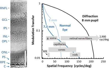
Fig. 61.6
(left) Histological cross section of primate retina with labels and scale bar (100 μm) added. (Cross section is reproduced with permission from the Royal Society of London [66].) (right) MTF of the eye under normal viewing is shown with pupils that are 3 and 7.3 mm in diameters and with the best refraction achievable using trial lenses averaged across 14 eyes. Also shown is the diffraction-limited MTF for the 8 mm pupil. The area between the normal and diffraction curves represents the range of contrast and spatial frequencies inaccessible with a normal eye, but reachable with AO. Also indicated is the range of fundamental frequencies defining several clinically important cell-sized structures. The ganglion soma (g. soma) range corresponds to sizes in the foveal margin and superior periphery with mean diameters of 11.7 μm (25.6 cyc/deg) and 15.8 μm (19 cyc/deg), respectively [67]. Individual retinal nerve fibers can get as large as 3.9 μm (75 cyc/deg), but the most probable axon diameter is about 0.45 μm (660 cyc/deg) [68]. Retinal capillary diameters are shown for central retina with mean size of 4.9 μm (61.2 cyc/deg) [69]. Cone row-to-row spacing (derived from cone density) is shown for the central +/−15°, averaged over the four meridians [70]. Rod row-to-row spacing is shown for 4.5 and 17° retinal eccentricity, again from histology [70, 71]. RPE spacing is shown for 5–20° in the superior retina [72]. Key: RNFL retinal nerve fiber layer, GCL ganglion cell layer, IPL inner plexiform layer, INL inner nuclear layer, OPL outer plexiform layer, ONL outer nuclear layer, PS photoreceptor segments, RPE retinal pigment epithelium, C choroid
61.3 Adaptive Optics
An ophthalmic AO system consists of the same principle components as those employed in ground-based telescopes: wavefront sensor, wavefront corrector, and control system. These components are highlighted in the simplified AO schematic of Fig. 61.7 (see figure caption for details). The wavefront sensor and corrector operate in closed loop, and the correction imparted on the wavefront is based on the wavefront sensor measurement. The effectiveness of these components depends fundamentally on their ability to measure, correct, and track ocular monochromatic aberrations, the extent to which depends strongly on the spatial and temporal properties of the aberrations as described in the previous section. General ophthalmic requirements for these (measure, correct, and track) are presented here.
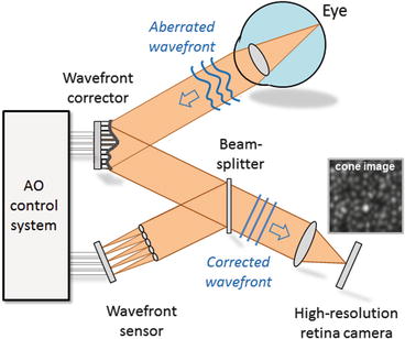
Fig. 61.7
Concept schematic of AO applied to the eye. The wavefront sensor (shown here as a Shack Hartmann implementation) works by measuring the reflection of a light beam that is focused onto the subject’s retina. The reflection is distorted as it passes back through the refracting media of the eye. A two-dimensional lenslet array, placed conjugate with the eye’s pupil, samples the exiting wavefront forming an array of images of the retinal spot. A CCD or CMOS sensor records the displacement of the spots, from which first local wavefront slopes and then global wavefront shape are determined. Wavefront compensation is realized with a deformable mirror. The mirror lies in a plane conjugate with the subject’s pupil and the lenslet array of the SHWS. For retinal imaging, a light source (not shown) illuminates the retina, some of which is reflected out of the eye, reflects from the wavefront corrector, and forms an aerial image at the retina camera
61.3.1 Wavefront Sensor
There is an abundance of optical sensors for wavefront measuring with many representing highly mature devices. These include the Shack-Hartman wavefront sensor (SHWS), shearing interferometer, pyramid sensor, curvature sensor, phase diversity, laser ray tracing, phase-shifting interferometer, and common-path interferometer. While several of these have been applied to the eye and others continue to attract interest, to date almost all operational AO systems for the eye have been constructed using the SHWS. As such, we confine our attention to this sensor type, though much of which will be applicable to the other sensors.
A first-order design of the SHWS entails evaluation of four key properties: (1) spatial sampling, (2) dynamic range, (3) accuracy, and (4) signal to noise. These are set primarily by the characteristics of the lenslet and CCD/CMOS arrays of the sensor, and therefore, selection of these two components is critical. Spatial sampling of the sensor is specified by the number of lenslets that fills the pupil of the eye. The necessary number of lenslets for reliable representation of the ocular aberrations depends on the composition of the ocular aberrations, pupil size of the eye, and to a lesser extent the SH wavelength. A general rule of thumb is that one lenslet is required for every Zernike mode that is to be measured. Based on this, reliable representation up through tenth Zernike order requires at least 63 lenslets that uniformly cover the pupil. In practice, SHWSs routinely sample the pupil with much higher density. There is little cost to do so since there is an abundance of light for the sensor. Oversampling makes the measurements more robust (to pupil edge effects, eye motion, drying of the precorneal tear film, and system noise) and applicable to eyes with a wider range of aberrations. Schematic of the SHWS is shown in Fig. 61.8.
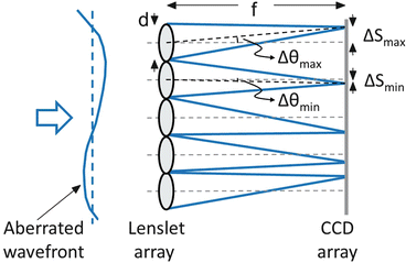
Fig. 61.8
Schematic illustrates the principle operation of the Shack-Hartmann wavefront sensor
Dynamic range refers to the maximum wavefront slope, Δθ max, that can be measured by the SHWS. Δθ max is typically expressed as ΔS max/f, where ΔS max is the maximum displacement of the lenslet spot (=lenslet radius) and f the lenslet focal length. Since spherical and cylindrical refractive errors typically consume much of the dynamic range of the sensor, it is often more useful to convert ΔS max to a maximum measurable defocus (diopters), expressed by D = Δθ max/ (pupil radius). For example, a lenslet diameter of 0.4 mm and a lenslet focal length of 24 mm give a Δθ max and D of 8.3 mrad and 2.44 diopters, respectively, for a 6.8 mm eye pupil. In general, the dynamic range can be increased by increasing the lenslet diameter, decreasing the lenslet focal length, or decreasing the pupil diameter.
Accuracy refers to the minimum wavefront slope, Δθ min, that can be measured by the SHWS. Δθ min is expressed as ΔS min/f, where ΔS min is the minimum detectable displacement of the lenslet spot. ΔS min depends on the pixel size of the SHWS detector, diameter of lenslet spot at the detector (which is a function of the lenslet diameter and focal length), accuracy of the centroiding and thresholding algorithms, and signal to noise of the captured SHWS spot image. In general, sub-pixel accuracy is routinely achieved [73]. While the SHWS parameters can be manipulated to increase accuracy, dynamic range of the sensor also depends on the lenslet diameter and focal length, but inverse of that for accuracy thereby creating a clear trade-off between these two SHWS properties. This trade-off can be partly avoided with smarter centroiding algorithms. For example, cross-correlation techniques have been used to locate centroids of spots outside the conventional search box area. This approach – which is employed in some commercial wavefront sensor systems – substantially increases the dynamic range of the system without loss in accuracy.
Signal to noise of the captured SHWS spot images is limited by the amount of light that can be safely directed into the eye, number of pixels per lenslet focal spot, quantum efficiency of the SHWS detector, and throughput efficiency of the SHWS. Fortunately, ophthalmic AO systems operate under relaxed light requirements, certainly well above the ∼100 photons/lenslet needed to close astronomical AO loops. A typical ophthalmic AO system, running at tens of milliseconds exposure time, has at least ∼500,000 detected photons/lenslet, this with hundreds of lenslets that sample the pupil. Such high light levels permit use of relatively low quantum efficient CCD and CMOS detectors and tens of pixels that sample the core.
61.3.2 Wavefront Corrector
The effectiveness of AO to correct ocular aberrations has historically been limited by the performance of the wavefront corrector, the most expensive AO component. This device dynamically imparts an ideally conjugate aberration profile onto the incident wavefront, thus canceling the original aberrations.
Wavefront correctors first applied to the eye were developed primarily for compensation of atmospheric turbulence, a common example being macroscopic discrete actuator deformable mirrors (DMs), such as those manufactured by Xinetics, Inc. [74]. Specifically, their actuator number, stroke, influence function, and speed were tailored to the spatial and temporal properties of the atmosphere [75] rather than that of the eye [33, 34, 51, 52]. Stroke refers to the dynamic range of the corrector and limits the largest wavefront error that can be corrected. Larger stroke provides better correction of large-magnitude aberrations. Actuator number across the eye’s pupil and actuator influence function (localized deflection of the mirror surface that results when a single actuator is pushed or pulled) determine the fidelity of the correction. More actuators and a more localized influence provide better correction of high-spatial-frequency aberrations, i.e., aberrations of high order. The dynamic range of these first devices did not match that needed for the eye and provided incomplete compensation of ocular aberrations. Also, their kilohertz response was overkill for the 1–2 Hz fluctuations of the ocular aberrations, and the devices themselves were generally bulky, with large mirror surfaces (∼several centimeters or more) that required long focal length relay optics to magnify the pupil of the eye.
Since then, there have been several extensive theoretical studies that have evaluated the performance of general wavefront corrector classes [76, 77] as well as specific commercial devices [78, 79]. These studies along with empirical evaluations have helped define corrector parameters for eye use, in particular the required actuator stroke, number, and influence function. Other important corrector parameters include temporal response, surface reflectivity for broadband use, corrector diameter, and of course cost.
In recent years, an expanding array of alternative wavefront corrector technologies has flooded the market, replacing the previous small market driven by atmospheric turbulence applications. These new technologies have been a welcome relief, generating a range of commercial devices that span all four major corrector classes: segmented, discrete actuator, bimorph, and membrane wavefront correctors. Figure 61.9 shows representative devices from the four classes that have been applied to the eye. These new devices provide substantially improved corrector performance specifically in the areas needed for ocular applications. Additionally, their small mirror footprint and lower cost are enabling AO technology to jump from the vision research laboratory to the clinic and into turnkey commercial AO ophthalmic cameras.
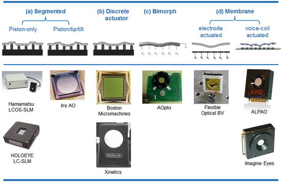
Fig. 61.9
Four main classes of wavefront correctors with specific devices that have been applied to the eye. (a) Piston-only segmented correctors consist of an array of small planar mirrors whose axial motion (piston) is independently controlled. Liquid-crystal spatial light modulators control the wavefront in a similar fashion, but use changes in refractive index rather than physical displacement of a mirror surface. Piston/tip/tilt segmented correctors add independent tip and tilt motion to the piston-only correctors. (b) Discrete actuator deformable mirrors consist of a continuous, reflective surface and an array of actuators, each capable of producing a local deformation in the surface. (c) Bimorph mirrors consist of a layer of piezoelectric material sandwiched between a continuous top electrode and a bottom, patterned electrode array. A top mirrored layer is added to the top continuous electrode. An applied voltage causes a deformation of the top mirrored surface. (d) Electrode-actuated membrane mirrors consist of a grounded, flexible, reflective membrane sandwiched between a transparent top electrode and an underlying array of patterned electrodes, each of which is capable of producing a global deformation in the surface. Voice-coil actuated membrane mirrors provide similar global deformation, but realized with miniaturized voice-coil actuators that make no contact with the membrane. Note that photographs of the devices are not shown to scale
61.3.3 Control System
The control system performs the critical step of rapidly and repeatedly converting the raw output of the wavefront sensor into voltage commands that shape the corrector surface, i.e., the deformation created by the sum response of the corrector actuators. The control loop takes into account the number, arrangement, and interaction of lenslets and actuators; the influence function and stroke of actuators; temporal response of the AO components; and a desired performance criteria, e.g., minimize the RMS wavefront error. The control loop can be characterized in terms of its spatial and temporal properties.
Spatial (static) control starts with the layout of lenslets and actuators. Typical AO systems for the eye sample each actuator with two to ten lenslets. This oversampling increases the tolerance to alignment errors and permits detection of all corrector modes. Spatial control of the wavefront corrector using the wavefront sensor is normally realized (based on a linear systems approach) by a multiplication of two matrices, one representing the wavefront sensor output, S, (slope measurements) and the other a reconstructor matrix, A + , representing the interaction of each actuator with each lenslet (control matrix). This single matrix multiplication,

provides the voltages, V, that are applied to the corrector actuators. This approach – commonly referred to as the direct slop method – is fast and efficient. Another common approach is based on modal reconstruction in which wavefront slope measurements are converted to Zernike aberration modes (or other modal set) that in turn are converted to applied voltages. This approach allows explicit control of individual modes, including which ones are sent to the corrector.
(61.1)
Because of the high demand on corrector performance, a recent control strategy has been to distribute the demand across two wavefront correctors using a woofer-tweeter concept. In this arrangement, a large-stroke wavefront corrector (woofer) corrects large-amplitude, low-order aberrations and a high-spatial fidelity wavefront corrector (tweeter) corrects low-magnitude high-fidelity aberrations [25, 80–84]. However, mirror technology is catching up. New voice-coil-actuated membrane deformable mirrors offer both large stroke and relatively high number of actuators and have demonstrated comparable performance to that of woofer-tweeter systems [85].
Spatial properties, however, do not fully characterize the control system as they do not capture the closed-loop performance of AO. Specifically, they neglect the temporal dynamics of the ocular aberrations and the time delays associated with measuring the wavefront slopes and computing and applying the control voltages. Taking into account these temporal effects is critical for optimizing system performance and is accomplished by modeling temporal control as a cascade of transfer functions, each representing an independent component of the system. Details of this process are illustrated in Fig. 61.10 (top) using a block diagram representation of the AO control loop. As an example of the utility of the transfer function approach, Fig. 61.10 (bottom) shows predicted and measured traces of the power rejection magnitude (derived from the transfer functions) for representative AO configurations, one being five times faster than the other. The power rejection magnitude permits determining the cutoff frequency of the AO system, being defined as the frequency at which the power rejection magnitude first reaches 1. For the two configurations in Fig. 61.10, cutoff frequencies occur at 0.5 and 2.0 Hz, with the former consistent with the experimental measurements shown. Note that a cutoff of 0.5 Hz indicates that temporal frequencies below 0.5 Hz are (at least partially) corrected by the system, while those above 0.5 Hz are (at least partially) amplified. Because the vast majority of the aberration power in the eye lies below 1–2 Hz (see Fig. 61.3b), the 2.0 Hz bandwidth AO configuration should be adequately fast and provide improved performance over the 0.5 Hz system.
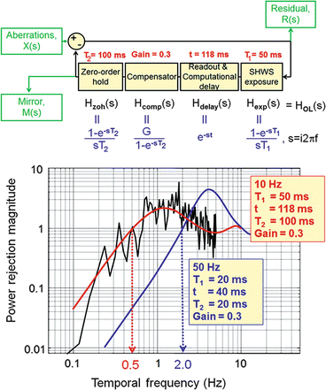
Fig. 61.10
(top) Block diagram of the AO system for modeling temporal performance. Input/output parameters M(s), X(s), and R(s) depict the time-varying aberrations of the eye, residual aberrations after correction, and wavefront corrector voltages. For temporal analysis, the AO system is decomposed as a linear cascade of independent transfer functions, in this case the four AO stages that most often limit temporal performance in ophthalmic AO systems: SHWS exposure, sensor readout and computation of V, integral compensator, and finally holding mirror position for one AO loop period. T 1 is the exposure duration of the SHWS detector, T 2 is the sampling period of the AO loop, and t is the total delay to readout the sensor and compute V. (bottom) Experimental and theoretical curves for the power rejection magnitude of an ophthalmic AO system. Experimental curve (jagged, black line) was obtained on one eye using a gain of 0.3 for a 6.8 mm pupil. The corresponding theoretical curve (solid, red) was based on the actual system parameters given in the leftmost box on the plot. The second theoretical curve (blue) predicts the performance of an AO system that is five times faster. System parameters are given in the rightmost box
Finally, it is worth mentioning that there is growing interest in wavefront sensorless control of AO systems for imaging biological structures for which AO cannot establish a reliable wavefront that can be corrected by a wavefront corrector. Bonora et al. have recently published a short review of wavefront sensorless techniques including demonstration of a wavefront sensorless AO-OCT system [86]. Future refinements of this technique, beyond the simple implementation presented in their chapter, should allow its extension to in vivo applications. Interestingly an example of sensorless adaptive optics scanning laser ophthalmoscopy (AO-SLO) for imaging in vivo human retina has been recently presented [87].
61.4 Adding AO to OCT
61.4.1 AO Benefits
AO permits access to the full retinal reflection that exits a large pupil of the eye (>6 mm). This translates into three technical benefits for OCT that improve the visualization and detection of microscopic structures in the retina: (1) higher lateral resolution, (2) a smaller lateral speckle size, and (3) higher collection efficiency for light backscattered from the retina. Of these three, lateral resolution has received considerably the most attention, but the other two add significant performance value. The benefit of each is discussed below.
The addition of AO typically increases the lateral resolution by approximately six times over commercial OCT. Of course to take advantage of this resolution requires increased A-scan sampling so that the closeness of the individual A-scans does not compromise the improved optical resolution. Current state-of-the-art adaptive optics, ultrahigh-resolution OCT (AO-UHR-OCT) has an isotropic 3D resolution of 2.5 × 2.5 × 3 μm3 (width × length × depth) in retinal tissue. Two of these three dimensions are governed by conventional optics (diffraction and aberrations), and therefore, the resolution volume is highly sensitive (goes as the square) to AO performance and actually more so than OCT that acts only on a single dimension, depth. Figure 61.11 compares the size of this 3D resolution element of AO-UHR-OCT (smallest black symbol) to that of OCT without AO and to that of two other major imaging modalities – confocal scanning laser ophthalmoscope and flood illumination – with and without AO. As shown, the addition of AO to UHR-OCT or commercial OCT improves the resolution volume by 36 times. Furthermore, AO-UHR-OCT has a resolution volume that is 72 times better than that of commercial OCT, taking into account AO and the two times improvement in axial resolution afforded by the wider source spectrum. In general, AO-UHR-OCT provides the best resolving capability of any of the imaging modalities and the only instrument able to resolve cells in all three dimensions.
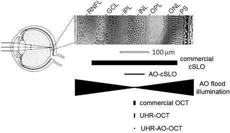
Fig. 61.11
Comparison of (top) cell size in a histological cross section of the human retina to (bottom) the resolving capability of the major types of retinal imaging modalities with and without AO. The vertical and horizontal dimensions of the solid black symbols denote, respectively, the lateral and axial resolution of the instruments. Examples shown include the commercial confocal scanning laser ophthalmoscope (cSLO), adaptive optics with confocal scanning laser ophthalmoscope (AO-cSLO), adaptive optics flood illumination, commercial OCT, ultrahigh-resolution OCT (UHR-OCT), and adaptive optics with ultrahigh-resolution OCT (AO-UHR-OCT). See key in Fig. 61.6 for retina labels (Reproduced with permission from The Royal College of Ophthalmologists, Ref. [27])
The second benefit of AO is reduced lateral speckle size. The interferometric nature of OCT generates high-contrast speckle that permeate the entire OCT image and masks structural details, especially those at the resolution limit of the system. Since lateral speckle size is inversely related to pupil (beam) diameter, the larger pupil size afforded with AO (>6 mm) reduces theoretically the lateral dimension of speckle. For current state-of-the-art UHR-AO-OCT, this corresponds to a reduction of roughly six times and a corresponding speckle volume of 36 times compared to that of standard commercial OCT. Cense et al. [88] confirmed this improvement by a speckle analysis of B-scans acquired 3° from the foveal center. In Fig. 61.12, two examples are given, without (1.2 mm beam) and with (6.0 mm beam) AO. Analyzed over many B-scans, the FWHM lateral speckle diameter was equal to 14 ± 1 μm (1.2 mm beam) and 3.1 ± 0.1 μm (6.0 mm beam), consistent with the calculated FWHM diffraction-limited airy disk sizes of 14 and 3 μm, respectively.
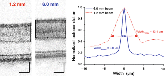
Fig. 61.12
(left) B-scans of the same retinal patch taken with the same AO-OCT system, but with 1.2 mm and 6.0 beams. Focus of the AO was near the outer plexiform layer; wavelength was 840 nm. (right) The FWHM lateral width of speckle was determined from the width dimension of the two-dimensional autocorrelation of the demarcated area in the B-scans. Only the upper retinal layers were included in the analysis because the autocorrelation algorithm was sensitive to abrupt changes in intensity (Reproduced with permission from OSA, Ref. [88])
This reduction in speckle size noticeably improves the appearance of the OCT image when magnified as illustrated by the commercial OCT and UHR-AO-OCT examples of Fig. 61.13. At the magnification shown, the B-scan in Fig. 61.13b has a photographic-like quality that shows clear delineation of the various neuronal layers. Speckle appears largely absent and certainly inconsequential for examining the retinal features visible in the image. Magnification necessary to view the microscopic features (see Fig. 61.13c), however, presents a very different view. Speckle and image blur are now obvious artifacts and mask retinal features that would otherwise be present in the image. This is particularly evident by comparing B-scan acquired with commercial system Spectralis (Heidelberg Engineering, Heidelberg Germany) (Fig. 61.13c) to the AO-UHR-OCT B-scan (Fig. 61.13d), which is of essentially the same patch of retina. Although maximum lateral resolution and structural detail are confined to the depth of focus (∼60 μm) that straddles the focal plane (which is at the retinal nerve fiber layer in the figure), speckle is noticeably smaller throughout the entire image. Thus most of the visual difference between the commercial OCT and UHR-AO-OCT B-scans is due to differences in speckle size. Based on the autocorrelation insets, the lateral dimension of speckle is 5× smaller (because of AO) and the axial dimension of speckle roughly 2× smaller (because of UHR-OCT).
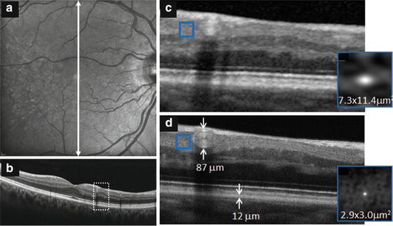
Fig. 61.13
Comparison of fast B-scans acquired of the same patch of retina of a 62-year-old subject with Heidelberg Spectralis and AO-UHR-OCT systems [89]. Spectralis images are shown for (a) 20° fundus view and (b) vertical B-scan that traverses the fovea. Region highlighted by the white, dashed box (3° wide) is magnified and displayed in (c). The highlighted region crosses an arcuate RNFL defect. AO-UHR-OCT B-scan is shown in (d). Both Spectralis and AO-UHR-OCT images are an average of 7 fast B-scans, the UHR-AO-OCT with 0.9 μm spacing. The averaging is consistent with the default averaging mode of the Spectralis system, for a fairer comparison. Insets show the autocorrelation (gray scale map) for the region inside the superimposed box in (c, d), respectively (Reproduced with permission from Elsevier, Ref. [89])
A larger pupil and wider spectral light source decrease the lateral and axial dimensions of speckle, but further improvement in AO-OCT image clarity can be gained by reducing contrast of the speckle. Figure 61.14 shows one such example [25]. Because retinal nerve fiber bundles (RNFB) on the local level share the same orientation, averaging of adjacent B-scans (which are orthogonal to the bundle direction) is used to reduce speckle contrast without sacrificing spatial information of the RNFB cross section (width and thickness). Thus bundle clarity is improved as shown in the figure.
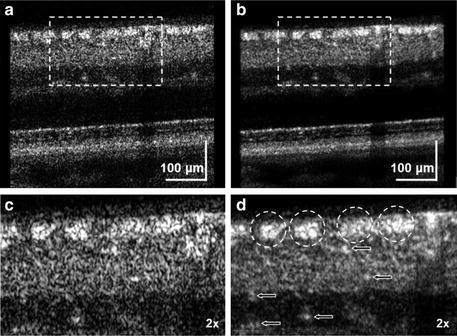
Fig. 61.14
Comparison of (a) single and (b) averaged B-scans obtained with AO-UHR-OCT system. AO focus was set at inner retina layers at 9° S 4.5° NR eccentricity of healthy 55-year-old volunteer. Dashed rectangles in a and b correspond to the magnified regions shown in c and d, respectively. Averaging was over ten AO-UHR-OCT frames. Dashed circles indicate location of the nerve fiber bundles. Arrows indicate location of micro capillaries in the inner retina. Note improved visibility of retinal nerve fiber bundles with averaging (Reproduced with permission from OSA, Ref. [25])
The third benefit of adding AO to OCT is the higher collection efficiency for light backscattered from the retina, which translates into higher SNR. In theory a gain of approximately 8–12 dB is expected, based on the difference in pupil size between conventional OCT and AO-OCT systems and the angular distribution of reflected light expected due to the Stiles-Crawford effect. This effect originates in photoreceptors, typically the brightest layer in the retina and therefore influences SNR [90]. Our measurements approach this theoretical estimate. Specifically, the comparison between measurements taken with the 1.2 mm beam without AO and the 6.0 mm beam with AO (based on Fig. 61.12 setup) demonstrated an increase in dynamic range of at least 4 dB. This number can be further increased by an estimated 4 dB when the AO system is focused at a highly reflective layer, such as the photoreceptor or RPE, as opposed to the inner plexiform layer that was used in the experiment. Adding these numbers, the total gain was 8 dB [88].
61.4.2 AO Disadvantages
AO in OCT is attractive because of the improved resolution, reduced speckle, and increased sensitivity, but these come at a cost. Pragmatic ones include increased system complexity, physical size, and expense. Along with these though are fundamental performance disadvantages, two principle ones being reduced depth of focus, and increased sensitivity to chromatic aberrations, both caused by the larger pupil size.
Depth of focus is inversely related to pupil size and trades-off with lateral resolution. Figure 61.15 shows this fundamental trade-off for an unaberrated eye, in this example at a wavelength of 800 nm. Using the pupil sizes in the AO-OCT example of Fig. 61.12, a 1.2 mm pupil provides a transverse resolution of 13.6 μm and a depth of focus of 1.45 mm. The depth of focus exceeds the retinal thickness by several times, making all retinal layers equally in focus, but at inadequate resolution to resolve cells. Increasing the pupil diameter to 6 mm increases the transverse resolution sufficiently for single-cell imaging (2.7 μm), but at the expense of a much narrower depth of focus, just 58 μm. This depth of focus barely covers a single neural layer in the retina (see Fig. 61.15) and thus precludes imaging the full retina thickness simultaneously and necessitates careful focusing of a single layer of interest, for example, photoreceptor segments. Such axial restriction clearly undermines the power of most OCT modalities that rapidly acquire information in depth (A-scans), either simultaneously as in SD-OCT or nearly so as in swept source OCT.
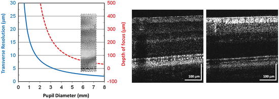
Fig. 61.15
(left) Transverse resolution (solid, blue) and depth of focus (dashed, red) as a function of pupil diameter for an unaberrated eye. Resolution at the focal plane is defined by 1.22 λf e /d, where λ is the wavelength of light (800 nm), f e is the focal length of the eye (16.7 mm), and d is the pupil diameter. Assuming a Gaussian beam intensity profile, depth of focus is specified as two times the Rayleigh range. (right) Example of narrow depth of focus of an AO-UHR-OCT system [89]. B-scans were acquired of the same retinal location with AO focus at the photoreceptor segments (left) and retinal nerve fiber bundles (right). Shift in focus was 0.4 Diopters, which was generated by the AO wavefront corrector (Reproduced with permission from Elsevier, Ref. [89])
While high lateral resolution and large depth of focus cannot be realized simultaneously with conventional optics, methods to optimize this trade-off are well established in the optics literature albeit showing limited success. These methods are just beginning to be applied to AO-OCT systems [91]. Non-conventional approaches that take advantage of the phase information intrinsic in the OCT image offer considerably more promise. These approaches have been demonstrated to remove focus blur and other aberrations in post-detection, though under well-controlled conditions and specialized samples [92]. While promising, major questions remain as to their robustness to work in living tissue such as the eye.
Another fundamental performance disadvantage of AO is that it increases the sensitivity of OCT to chromatic aberrations. As discussed in Sect. 61.2.2 and shown in Fig. 61.5, the human eye has significant chromatic aberrations. Recent work by Fernández and Drexler [93] has shown that ocular chromatic aberrations can significantly decrease the detected signal and degrade the lateral resolution of AO-OCT, the extent to which depends strongly on the spectral bandwidth of the OCT source and pupil size. Figure 61.16 illustrates this dependence, plotting Strehl ratio of the eye as a function of pupil diameter (1–8 mm) and spectral bandwidth (40–200 nm). The plot shows image quality monotonically decreases with pupil size and bandwidth. At small pupil sizes typical of conventional OCT (<2 mm), Strehl ratio is negligibly impacted by chromatic aberrations regardless of the bandwidth, even 200 nm. However, at pupil sizes useful for AO (>6 mm), lateral resolution noticeably drops for bandwidths that exceed that of standard OCT (>40 nm). For bandwidths used in UHR-AO-OCT (>100 nm), image quality is predicted to fall below a Strehl of 0.5, this all with perfect AO correction of monochromatic aberrations. Thus given the typical bandwidths of OCT sources, and especially those for UHR-OCT, the benefit of AO correction of monochromatic aberrations is only useful if the chromatic aberrations are corrected too. The present solution is to insert a customized achromatizing lens into the AO-OCT sample arm to provide a fixed correction of the expected average chromatic aberrations in the human eye. Numerous labs have reported such lenses and have demonstrated improvement in image quality [83, 94, 95]. The design of one such lens is shown in Fig. 61.16b; its effectiveness to compensate chromatic aberrations in five subjects is validated in Fig. 61.16c [96].
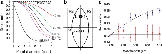
Fig. 61.16
(a) Polychromatic Strehl ratio of the human eye computed as a function of pupil diameter at the eye and spectral bandwidth of the imaging light source. Colored, solid lines depict perfect correction of ocular monochromatic aberrations, thus image quality is limited by diffraction and chromatic effects. Black, dashed line depicts perfect correction of both monochromatic and chromatic aberrations of the eye. Black, solid line depicts average of four real eyes with all aberrations present (Reproduced with permission from OSA, Ref. [93]). (b) Customized achromatizing lens for correction of ocular chromatic aberrations in the near infrared. (c) Chromatic difference of refraction (defocus) in the near infrared with and without the achromatizing lens (red and blue color, respectively) shown in (b). Error bars depict the standard deviation of measurements on five subjects. The black, dashed line is the predicted curve for the human eye, the near-infrared portion of that shown in Fig. 61.5. The dotted line denotes perfect chromatic correction (Reproduced with permission from OSA, Ref. [96])
Achromatizing lenses are critical for correction of LCA in the eye, but provide no benefit for TCA, which can be substantial and can dilute the benefit of the LCA and AO correction. Zawadzki et al. [25] recently investigated theoretically and experimentally the impact of the eye’s LCA and TCA on the performance of high-resolution retina cameras and strategies to minimize them. They determined the extent to which TCA impacts retinal imaging and the conditions under which it can be held at acceptable levels. As discussed in their paper, the two primary contributors of TCA for retinal imaging are (1) errors in the lateral positioning of the eye, h, relative to the optical axis of the retina camera and (2) off-axis imaging, φ, i.e., imaging away from the achromatic axis of the eye. Two of their key results are shown in Fig. 61.17. The left plot shows the predicted TCA as a function of lateral displacement of the eye’s nodal point from the camera’s optical axis. Larger displacements as well as wider source spectra are predicted to generate larger TCA. Use of a pupil camera and bite-bar stage permits accurate positioning of the subject’s pupil, likely within about ±0.5 mm. This precision of pupil alignment should be sufficient to keep TCA at acceptable levels. However, clinical use of AO-OCT ultimately means replacing the bite-bar stage with a chin and forehead rest. For these instruments, larger positioning errors are expected.
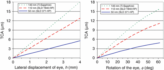
Fig. 61.17
Modeling of TCA as a function of (left) lateral misalignment of the eye, h, and (right) off-axis imaging, φ. (Left) TCA is plotted as a function of lateral displacement of the eye’s nodal point relative to the optical axis of the retina camera. (Right) TCA is plotted as a function of eye rotation (defined as the angle between the camera’s optical axis and the eye’s achromatic axis). The eye’s entrance pupil remains centered on the camera’s optical axis, which is a common experimental alignment protocol. Three near-infrared bands were chosen that correspond to specific OCT light sources (Reproduced with permission from OSA, Ref. [25])
Figure 61.17 (right) shows the predicted TCA for off-axis imaging when the eye’s entrance pupil remains centered on the camera’s exit pupil. The figure shows that larger rotations as well as wider source spectra lead to larger TCA. As an example for the SLD T840-HP source (UHR-AO-OCT), the TCA remains below 3.5 μm up to ±16° of rotation. This suggests that the central portion of the retina – from the fovea out to about the optic disk – can be imaged with this source with relatively small TCA. This interpretation assumes the achromatic axis intersects the retina near the fovea. The 50 nm source will allow even larger rotation (±39°), while the 140 nm less (±11°). Perhaps of most importance, these predictions represent fundamental limits on the accessibility of the microscopic retina with AO-OCT. The exact numbers will change depending on source spectrum, eye alignment, pupil size, and chromatic aberrations, but hard limits exist and impose serious consequences on imaging performance.
61.5 Examples of AO-OCT Systems
Not surprisingly, development of AO-OCT systems has closely followed advances of the underlying AO and OCT technologies. For AO, these advances have largely been in improved componentry (wavefront sensors and correctors), optical designs (aberration free), and control algorithms that better account for the unique properties of the eye. While considerable AO advances have occurred in these areas, the basic configuration of ophthalmic AO has remained unchanged, being based on the same three components: wavefront sensor, wavefront corrector, and control algorithm.
In contrast, OCT has progressed rapidly along several different design configurations, each taking advantage of different key technologies, especially those for light generation and detection. Major development of these configurations occurred more or less sequentially, and thus AO-OCT development has mirrored these transitions. Over the last nine years, all major OCT design configurations have been demonstrated with AO. AO-OCT combinations include time-domain en face (xy) flood-illumination OCT using an areal CCD, time-domain tomographic scanning (xz) ultrahigh-resolution OCT, time-domain en face scanning (xy) OCT, high-resolution spectral-domain OCT, ultrahigh-resolution spectral-domain OCT, and more recently swept source OCT.
Regardless of design configuration, AO-OCT performance has been commonly assessed using standard AO and OCT metrics, but ultimately judged by the quality of the retinal image and retinal microstructure that is revealed. Consistent with the rest of the ophthalmic AO field, the retinal cell of choice to assess retinal image quality has been the cone photoreceptor. This is due in part to the cone’s high contrast in reflection, regular arrangement that varies predictively with retinal eccentricity and stratified 3D reflectance profile.
Here we present the major AO-OCT design configurations that have been developed, categorized broadly by time-domain and Fourier-domain types. Emphasis is on the first systems reported.
61.5.1 AO with TD-OCT
The first implementations of AO-OCT were based on TD-OCT, the method ubiquitous of OCT up to about 2004. This included a flood-illuminated version based on an areal CCD [16] and a conventional version based on tomographic scanning (xz) [17]. These first instruments demonstrated the potential of the combined technologies, but fundamental technical limits, primarily in speed, precluded their scientific and clinical use. Nevertheless they represented first steps toward more practical designs that became possible with new OCT methods. The one notable new time-domain method that has been combined with AO and continues to be developed is high-speed transverse scanning TD-OCT (TS-OCT) [22, 24].
Stay updated, free articles. Join our Telegram channel

Full access? Get Clinical Tree


