(37.1)
where the intensity variance is V I = (〈I 2〉 − 〈I〉2), and the delay-dependent function F(τ) is a decorrelation function that has contributions from many different dynamic processes in the cells and tissue. In the case of single scattering (QELS), it can be defined as a sum of independent exponential decorrelations as [26]
(37.2)
Typical time scales for scattering are related to the scattering vector and to the motion of the scatterer. For particles diffusing with a diffusion coefficient D, or drifting with a drift velocity v, the characteristic decorrelation times are
respectively, where the expression for drift is also equal to the Doppler frequency shift. Motions in living cells are not fast. Even molecules executing Brownian motion are hindered by the crowded molecular constituents of the cytoplasm [27]. Therefore, characteristic decorrelation times for light scattered from tissue range from many milliseconds to as slow as hundreds of seconds. This time frame is easily accessible with frame rates of common digital cameras.
(37.3)
When there are many processes that have characteristic times that are similar, the decorrelation function of Eq. 37.2 becomes difficult to separate into isolated contributions. It is then more convenient to work in the frequency domain by taking the Fourier transform of the dynamic imaging decorrelation function in Eq. 37.1. The mean-squared displacement of processes in biological systems is rarely by simple diffusion and commonly displays the signature of anomalous diffusion. Deviation from free diffusion is described phenomenologically through the relation
where D ∗ is a time-independent coefficient and t 0 is a characteristic time. The exponent for normal Fickian diffusion is β = 1. If β < 1, the diffusion is called subdiffusive, while if β > 1, the diffusion is called superdiffusive. Superdiffusive behavior occurs if there is persistent and correlated motion of the particle, as in the active transport of organelles. On the other hand, subdiffusive behavior is the most commonly encountered case when motion is constrained or impeded in some way, such as diffusion of molecules through the crowded cytosol.
(37.4)
Even in the presence of multiple scattering, dynamic light scattering information can still be extracted [28, 29] using diffusing wave spectroscopy (DWS) [30, 31] and an equivalent formulation of multi-scattering dynamic light scattering called diffuse correlation spectroscopy (DCS) [23, 25, 32, 33]. For multiple scattering in thick tissue, the effective squared scattering vector is
![$$ {q}_{eff}^2=4{k}^2\left[1+\frac{z}{l_s}\left(1-g\right)\right] $$](/wp-content/uploads/2017/03/A76297_2_En_38_Chapter_Equ5.gif)
where g is the anisotropy factor (typically g ≈ 0.9 in tissue), z is the coherence-gated depth in the tissue, and ls is the mean-free scattering length of a photon (typically l s ≈ 20 μm). Multiple scattering causes the effective squared scattering vector to increase linearly with depth from the value set by single backscattering. This has the effect of “speeding up” the light fluctuations from increasing depths.
(37.5)
In biological applications, DCS has been used to monitor tissue response to burns [34], brain activity [35], blood flow [24, 25] and tissue structure [36]. DCS uses high-coherence laser sources and measures the temporal diffusing field autocorrelation function. The primary uses have been for macroscopic measurements of blood flow, which has been validated through comparisons with Doppler flowmetry and ultrasound [37–39]. A technique related to DCS, but that more directly uses speckle imaging, is speckle contrast imaging (SCI) [24]. This technique is used primarily for imaging of vasculature in vivo because the fast motions of blood cells blur the speckle contrast in images acquired with a long exposure time [40].
Optical coherence tomography (OCT) forms images by scanning and rastering. Speckle in OCT has long been considered an unwanted side effect of the coherent imaging, and many approaches have been explored to reduce speckle [41–43]. However, speckle decorrelation also can be studied in OCT data to provide similar information as provided by DCS. This has been used to measure intracellular rheology [12] and diffusion [44] and to find dynamic signatures of apoptosis [45] and motion of mucosa [46]. OCT is used in a Doppler mode for blood flow detection [47, 48]. Motility contrast imaging (MCI) is a related tissue-scale functional imaging technique that uses subcellular motion as the imaging contrast [49–51]. Motility contrast imaging of live tissue is based on two principles: dynamic light scattering from the motions of the constituents of living cells and coherence-gated depth resolution [52] that isolates the motional signals from specific depths.
37.3 Motility Contrast Imaging of Living Tissue
In biodynamic imaging, the coherence gate is formed by a low-coherence light source detected by digital holography on a CCD camera chip [53] (see Chap. 31, “Interferometric Synthetic Aperture Microscopy (ISAM)”). Light scattered from a selected depth is recorded in the digital hologram. When dynamic light scattering and coherence gating are combined, intracellular motion can be measured volumetrically up to 1 mm deep inside tissue with a spatial resolution of tens of microns. The basic optical configuration for an optical coherence imaging (OCI) system is shown in Fig. 37.1. Low-coherence light is split at a beam splitter into a signal arm that illuminates the sample and a reference arm that has a variable-delay retroreflector. Light scattered from the sample intersects with the reference beam at the plane of the CCD electronic chip [54] with a small crossing angle of about two degrees. The selected depth is defined by the path length from the beam splitter to the CCD plane. The low-coherence light source is either a 100 fsec Ti:sapphire laser or a Superlum superluminescent diode, both operating at a center wavelength of 840 nm. The hologram is recorded on the CCD chip and is “read-out” by a digital Fourier transform algorithm, which is stored as a layer in a volumetric data set.
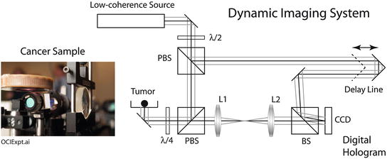
Fig. 37.1
Biodynamic imaging experimental setup that uses off-axis digital holography to capture dynamic speckle from a living tissue sample
A motility metric captures the general activity level of a living sample. The simplest motility metric is the normalized standard deviation (NSD) of fluctuating time-dependent speckle, which is also the temporal contrast
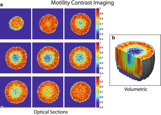
The NSD(x,y,z) motility metric is volumetric, with depth defined by the digital holographic coherence gate and the (x, y) coordinates of the image defined by reconstruction. An example of motility contrast imaging of a three-dimensional multicellular tumor spheroid is shown in Fig. 37.2 [50]. The spheroid is approximately 0.8 mm in diameter. The data are color coded according to the motility metric, with red signifying a high degree of motion and blue signifying a low degree of motion. For a spheroid of this size, the core is hypoxic and necrotic. The 200 μm thick proliferating shell is clearly discernible surrounding the less active core. The proliferating shell has high motility (red), and the necrotic core has low motility (blue).
(37.6)
Fig. 37.2
(a) False-color motility contrast image of an 800 μm-diameter tumor spheroid, showing the proliferating shell (red) and the necrotic core (blue). (b) Volumetric motility contrast image
Biodynamic imaging is a general imaging technique because it is responsive to intracellular motions, which occur in all living samples. Therefore, there are many potential applications for this new form of dynamic and functional imaging. Several of these are illustrated in Fig. 37.3. In (Fig. 37.3a) MCI is used to measure the activity of tissues from different cell lines, showing increasing activity from UMR-106 (rat osteogenic sarcoma), HT-29, and DLD-1 (human adenocarcinomas) to PaCa-2 (human pancreatic). A possible application in artificial reproductive technologies would be viability assessment of eggs and embryos prior to implantation in in vitro fertilization clinics. The motility activity of the central oocyte inside a cumulus-oocyte-complex (COC) is shown in Fig. 37.3b. MCI has been applied to tissue ex vivo as well, extending applications beyond purely in vitro culture. For instance, Fig. 37.3c shows the motility contrast between excised rat brain gray and white matter. Gray matter contains the cell bodies and is more dynamically active, while white matter consists primarily of axons. Figure 37.3d shows the margin between normal tissue and cancerous tissue in a mouse exgraft in which the cancerous tissue is more dynamically active than the normal tissue.
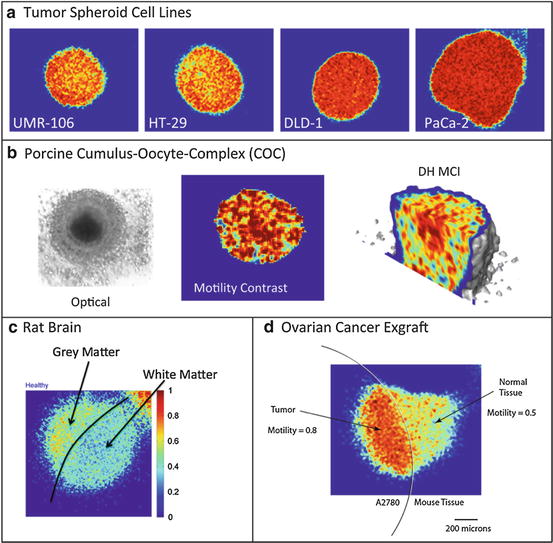
Fig. 37.3
Motility contrast images of (a) multicellular tumor spheroids derived from several different cell lines, (b) porcine cumulus-oocyte complexes, (c) white and gray matter of excised rat brain, and (d) cancer and normal tissue in a mouse ovarian cancer exgraft
37.4 Tissue Dynamics Spectroscopy and Drug-Response Spectrogram Fingerprints
The information received from coherence-gated light scattered from tissue relates to the many different types of motion that occur within cells across broad frequency ranges. It is possible to extend motility contrast imaging to tissue dynamics spectroscopy (TDS) by performing fluctuation spectroscopy to separate these motion contributions into partially overlapping frequency bands related to the different types of motion [55]. Tissue dynamics spectroscopy provides a label-free and noninvasive probe of cellular function and provides a functional assessment of drug candidates as a unique and new form of phenotypic profiling [7].
The Fourier transform of Eq. 37.1 under conditions of anomalous diffusion takes the form
![$$ S\left(\omega \right)=FT\left({A}_I\left(\tau \right)\right)=\frac{V_I}{\pi }{\displaystyle \sum_n\left[\frac{4}{\left(3-{\beta}_n\right)}\frac{f_n{\omega}_n^{\beta_n}}{\left({\omega}_n^{1+{\beta}_n}+{\omega}^{1+{\beta}_n}\right)}\right]} $$](/wp-content/uploads/2017/03/A76297_2_En_38_Chapter_Equ7.gif)
where β n is an anomalous diffusion exponent that is usually in the range β n ≈ 0.7–1.3.
(37.7)
Equation 37.7 retains the summation over the different dynamic processes taking place inside living tissue, and each process has a characteristic frequency ω n given by ![$$ {\omega}_n=\sqrt[\beta ]{q^2{D}_n^{*}/{t}_n} $$](/wp-content/uploads/2017/03/A76297_2_En_38_Chapter_IEq1.gif) . Because most motions in living cells are stochastic, even if they are actively driven by molecular motors consuming ATP, they can be described in terms of an effective (active) diffusion coefficient D n ∗ that describes different types of motion, such as vesicle or nucleus motion.
. Because most motions in living cells are stochastic, even if they are actively driven by molecular motors consuming ATP, they can be described in terms of an effective (active) diffusion coefficient D n ∗ that describes different types of motion, such as vesicle or nucleus motion.
. Because most motions in living cells are stochastic, even if they are actively driven by molecular motors consuming ATP, they can be described in terms of an effective (active) diffusion coefficient D n ∗ that describes different types of motion, such as vesicle or nucleus motion.An example of a fluctuation power spectrum from a tumor spheroid grown from the DLD-1 adenocarcinoma cell line is shown in Fig. 37.4. The baseline spectrum shows a knee frequency around 0.1 Hz with a slope around β ≈ 1. Two hours after 50 μM valinomycin is applied (a mitochondrial decoupler), the knee has shifted to 0.03 Hz with a smaller slope β < 1. Nine hours after the dose is applied, the spectrum has no clear knee frequency, and the slope is noticeably subdiffusive. Valinomycin reduces the mitochondrial membrane polarization (MMP) and suppresses the generation of ATP, thus significantly slowing the cellular metabolism. The shift of the spectrum to lower frequencies reflects this reduced metabolic activity, and the more subdiffusive slope may reflect a broader range of motional contributions.
Fig. 37.4
Power spectrum of DLD-1 adenocarcinoma tumor spheroid responding to 50 μM valinomycin. The spectra 2 h and 9 h after the dosing is compared to the baseline spectrum. The spectrum has three orders of magnitude of dynamic range and spans three decades of frequency from 0.005 to 5 Hz
The power spectrum of Eq. 37.7 changes as a function of time through the shift in the parameters Δω n (t), Δf n (t), and Δβ n (t). The changes can be small, which suggests the use of a differential spectral response defined by
This relative differential spectrogram captures the changes in spectral content as a function of time after a dose or a condition is applied. Tissue contains a wide range of characteristic frequencies producing complicated differential spectrograms.
(37.8)
An example of a tissue-response spectrogram is shown in Fig. 37.5 for pH 9 applied to rat UMR-106 osteogenic sarcoma tumor spheroids. The two-dimensional representation of the differential response is presented as relative frequency content change as a function of time. The treatment is applied at t = 0, and the tumor spheroids are monitored over 6 h. The times preceding the treatment show the system baseline. The spectrogram shows an initially high-frequency enhancement that decays over several hours. There is a sudden enhancement of low frequencies around 3 h after the change in pH.
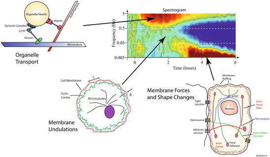
Fig. 37.5
The origin of spectroscopic motional signatures in a tissue-response spectrogram. The highest frequencies (around 5 Hz) relate to organelle transport, the mid-frequencies (around 0.5–0.05 Hz) to membrane undulations, and the lowest frequencies (around 0.005 Hz) to membrane forces and shape changes
The mechanistic interpretation of the tissue-response spectrogram is facilitated by considering the backscattering frequencies from dynamic intracellular processes. The general relationship for single backscattering under heterodyne (holographic) detection is q 2 D = ω D for diffusion, and qv = ω d for directed transport, where D is the diffusion coefficient, and v is a directed speed. The ranges in the parameters for directed transport and diffusion, respectively, are 0.006 < v < 2 μm/s and 4 × 10⁻⁴ < D < 0.1 μm2/s, set by the lowest and highest frequencies of 0.005–5 Hz. These are well within the range of intracellular motion in which molecular motors move organelles at speeds of microns per second [13, 56–59], although diffusion of very small organelles, as well as molecular diffusion, is too fast to be resolved by a frame rate of 10 fps. Membrane undulations are a common feature of cellular motions, leading to the phenomenon of flicker [60–64], and the characteristic frequency for light scattering from membrane undulations is in the range around 0.01–0.1 Hz [58, 61, 65]. The very low frequencies below 0.01 Hz relate to cellular rheology and the response of the cells to their local force environment, possibly including blebbing or the release of apoptotic bodies.
37.5 Phenotypic Profiling Based on Drug-Response Spectrograms
Cellular systems are highly complex, with high redundancy and dense cross talk among signaling pathways [66]. Biochemical target-based high-content screening can isolate single mechanisms in important pathways, but often fails to capture integrated system-wide responses. Phenotypic profiling, on the other hand, presents a systems-biology approach that has more biological relevance by capturing multimodal influence of therapeutics [67]. Ironically, phenotypic profiling is anachronistic, harking back to the days before genomics provided isolated targets. Nonetheless, it remains today one of the most successful approaches for the discovery of new drugs [68].
Most phenotypic profiling continues to be performed on two-dimensional culture, even though two-dimensional monolayer culture on flat hard surfaces does not respond to applied drugs in the same way as cells in their natural three-dimensional environment. This is in part because genomic profiles are different in primary monolayer cultures [69–71]. Several studies have tracked the expression of genes associated with cell survival, proliferation, differentiation, and resistance to therapy that are expressed differently in 2D cultures relative to three-dimensional culture. For example, three-dimensional culture display expression profiles more like those from tumor tissues than when grown in 2D [72–77]. In addition, the three-dimensional environment of 3D culture presents different pharmacokinetics than 2D monolayer culture and produces differences in cancer drug sensitivities [78–81].
Stay updated, free articles. Join our Telegram channel

Full access? Get Clinical Tree


