Fig. 81.1
(a) An OCT needle probe, consisting of a miniaturized side-viewing fiber-optic probe mounted inside a hypodermic needle with an imaging window near the tip. (b) Microscope image of a side-viewing fiber-optic probe designed for integration into a needle. SMF single-mode fiber, NCF no-core fiber, GRIN graded-index fiber. (c) Illustration of an envisaged OCT needle imaging system with a compact hand-held needle scanner
In this chapter, we will review the development and deployment of OCT needle probe technology and examine its use in preclinical and clinical applications.
81.2 Technology
Needle probes replace the sample-arm optics of a conventional OCT scanner. The tasks of the sample-arm optics are to scan and focus the incident light and to collect the weak backscattered light from the sample with high efficiency. Therefore, they define or significantly influence a number of key performance parameters of the OCT system, such as:
Transverse resolution
Depth of focus (DOF)
Sensitivity
Imaging speed
Losses or backreflections in the sample-arm optics will reduce the system sensitivity, whereas aberrations and alignment errors will negatively impact the transverse resolution and DOF. In a well-designed conventional free-space sample-arm setup consisting of a collimator, galvanometer mirrors, and a compound scan lens, minimal losses and diffraction-limited probe beam quality over the entire field of view can easily be simultaneously achieved using high-quality antireflection-coated optics. In the case of miniaturized sample-arm optics, such as those found in endoscopic or needle probes, the small dimensions and the available fabrication methods often force the probe designer to make trade-offs that negatively impact the performance of the OCT system. Recent advances in probe design and fabrication, however, have shown that needle probes can attain sensitivities and resolution comparable to bulk-optic sample arms [11].
81.2.1 Probe Optics
81.2.1.1 Probe Optics and Output Beam Parameters
The probe optics collimate or focus the diverging beam which is emitted from the single-mode fiber (SMF) of the OCT system and direct it into the sample, as illustrated in Fig. 81.2a. The focusing elements in the probe optics are typically realized using either GRIN optics or refractive optics. GRIN optics can be used either in the form of discrete GRIN rod lenses [12, 2] or in the form of short sections of multimode GRIN fiber that are directly fusion-spliced to the SMF [13–17, 11] in combination with coreless silica spacers made of no-core fiber (NCF). Due to its great importance for fiber probes, the use of GRIN multimode fiber as microlenses will be treated in more detail in Sect. 81.2.1.3. Examples of refractive optics are discrete ball lenses [8] or ball lenses that are directly formed on the end of fiber tips using fusion splicers [18, 12, 6]. Lensed fibers per se are not capable of imaging unless they are combined with some form of scanning mechanism, as will be discussed in Sect. 81.2.2. The most common scanning concept is rotation/pullback scanning in a side-facing configuration using a side-deflecting microreflector, as illustrated in Fig. 81.2a.
Fig. 81.2
Probe beam parameters. (a) Needle probe with a Gaussian output beam, using a GRIN lens which refocuses the beam emitted from the SMF into the sample volume. WD working distance, DOF R depth of focus using the Rayleigh range criterion, DOF 2 depth of focus using the factor-of-two criterion. (b) Needle probe with a wavefront-shaped output beam which is generated by a phase mask after the focusing optics. The beam features an extended DOF compared to a Gaussian but its transverse profile has sidelobes
This technique has its origins in catheter-based OCT systems [19, 20]. In side-facing configurations, complications due to astigmatism and beam distortion can arise if the beam must exit the needle through a nonplanar output interface (e.g., when an enclosing catheter or transparent casing is used). These issues will be addressed in the discussion of specific probe designs in Sects. 81.2.3 and 81.2.4. While the majority of OCT needle probes have Gaussian or Gaussian-like output beams (practical probes often exhibit beam distortion due to aperture diffraction and aberrations, as will be explained in Sect. 81.2.1.3), it has recently been shown that it is feasible to extend the depth of focus (DOF) of miniaturized fiber-based probes using phase masks [21, 22]. Such advanced probe designs utilizing probe optics with additional wavefront-shaping elements have non-Gaussian output beams that maintain an approximately constant central lobe diameter over a large axial distance in the focal region, as illustrated in Fig. 81.2b.
The axial and transverse resolutions of an OCT system are defined as the respective full-width at half-maximum (FWHM) of its three-dimensional (3D) point-spread function (PSF) [23, 24]. While the axial extent of the PSF is largely determined by the coherence length of the light source, the transverse extent of the PSF is determined by the intensity profile of the probe beam. For Gaussian probe beams, the 1/e2 diameter of the beam waist is sometimes quoted as the transverse resolution of the system even though this is not consistent with the widespread use of the FWHM in the axial direction. We prefer to adhere to the FWHM definition of the transverse resolution, which has the additional benefit of yielding more meaningful values for the central lobe diameters of aberrated or non-Gaussian output beams which may have sidelobes or pedestals that exceed relative levels of 1/e2. This is very important for the characterization of probe designs that use wavefront-shaping elements, such as phase masks, in order to generate focal regions with an extended DOF, as illustrated in Fig. 81.2b. For an ideal Gaussian profile, the FWHM transverse resolution is given by
where λ 0 is the wavelength in vacuum and NA is the numerical aperture. To define the DOF of the OCT imaging system, the double Rayleigh range is often used in the case of ideal Gaussian beams (see, e.g., [25]). The Rayleigh range criterion typically underestimates the perceived useful imaging depth range in OCT because a 40 % (factor of  ) change in transverse resolution is hardly visible due to the effects of logarithmic compression of the images and speckle. Similar to the reasoning for choosing the FWHM beam diameters to define the transverse resolution, we prefer to define the DOF as the range over which the FWHM beam diameter stays smaller than twice its minimum value in the focal region. This definition is more robust for numerically evaluating the DOF of probes that have wavefront-shaped output beams, which can have beam diameter variations within the useful imaging depth range that exceed a factor of
  , as illustrated in Fig. 81.2b. For an ideal Gaussian beam, the DOF according to the factor-of-two definition is simply a factor of
  larger than the DOF according to the Rayleigh range criterion:
where n is the sample refractive index and w 0 is the waist radius. We use the subscripts “2” and “R” to denote the DOF according to the factor-of-two or Rayleigh range criteria, respectively.
(81.1)
) change in transverse resolution is hardly visible due to the effects of logarithmic compression of the images and speckle. Similar to the reasoning for choosing the FWHM beam diameters to define the transverse resolution, we prefer to define the DOF as the range over which the FWHM beam diameter stays smaller than twice its minimum value in the focal region. This definition is more robust for numerically evaluating the DOF of probes that have wavefront-shaped output beams, which can have beam diameter variations within the useful imaging depth range that exceed a factor of , as illustrated in Fig. 81.2b. For an ideal Gaussian beam, the DOF according to the factor-of-two definition is simply a factor of larger than the DOF according to the Rayleigh range criterion:(81.2)
Another useful parameter for characterizing the output beam quality in the case of aberrated or wavefront-shaped output beams is the Strehl ratio S. The Strehl ratio of an aberrated system is defined as the ratio of its focal spot peak intensity to that of an equivalent diffraction-limited system [26]. Here, it allows the estimation of the penalty in the detected signal level (from a point scatterer) incurred by non-Gaussian output beams that are used to trade off a reduced focal spot intensity for an increased DOF. The Strehl ratio is difficult to obtain from measurements, but it can often be calculated by optical design software (e.g., it can easily be computed for simulated output beams obtained using the beam propagation method [22] which is described in Sect. 81.2.1.3), and therefore, it is mainly used as a figure of merit for optimization and comparison of probe designs. In the case of a simulated beam with a focal spot peak intensity  and total integrated beam power P, the Strehl ratio can be defined as [22]
where w Gauss is the 1/e2 waist radius of a suitably defined reference Gaussian beam (e.g., an ideal Gaussian beam with the same FWHM focal spot diameter as the simulated beam).
and total integrated beam power P, the Strehl ratio can be defined as [22](81.3)
81.2.1.2 ABCD Matrix Modeling
The optical design of micro-optic systems, such as miniaturized fiber-based probes for OCT, cannot generally be performed using the ray-tracing methods used in classical lens design because the approximations of geometrical optics are not satisfied (the size of the wavelength is no longer negligible compared to the dimensions of the optical elements, which means that diffraction effects will have a strong influence). Scalar wave theory is, therefore, required to properly simulate the propagation of the optical field through the optical elements of the probe. While several optical engineering software packages offer such functionality, they tend to be costly and complex to use. A simple but very effective alternative to a numerical scalar wave simulation is paraxial ABCD matrix transformations of Gaussian beams [27, 28]. Since the beam emitted by a SMF can be well approximated by a fundamental Gaussian mode [29], ABCD matrices can be used to calculate its transformation by the optical elements of the probe if these can be described sufficiently well by their paraxial, or first-order, optical properties (i.e., aberrations can be neglected). If no limiting apertures are present in the optics, this formalism fully accounts for diffraction and yields exact results within the regime of validity of the paraxial approximation, as the Gaussian beam is an exact solution of the paraxial wave equation [27]. Most optical beams used for OCT imaging lie well within the paraxial regime, which is a good approximation for beam divergence angles up to ∼30°, corresponding to a numerical aperture of ∼0.5 [27].
A very convenient feature of the ABCD matrix approach is that the Gaussian beam solution of the paraxial wave equation is separable in x and y, which means that independent complex beam parameters can be assumed in two orthogonal directions and that these can be transformed independently [27].
The ABCD matrix formalism lends itself to implementation in technical computing tools such as Matlab, making it ideal for fast and flexible design calculations. For this reason, ABCD matrix modeling has proven to be a useful framework for basic probe design and analysis [30, 15, 13, 16, 11] and as a simple tool for calculating approximate values for an optical design, which can then be experimentally optimized to yield the desired output beam characteristics. Furthermore, the possibility of working with astigmatic beams allows the study of the effects of astigmatism introduced by curved interfaces and to develop methods for its compensation [31, 16, 11, 32, 17]. As an example of the usefulness of the ABCD method, we will show in Sect. 81.2.4.1 how it can be used to derive a simple method for astigmatism compensation in needle probes [11] which exploits the “focal shift” effect that occurs when focusing at low Fresnel numbers.
While the ABCD matrix simulation method is a very useful tool for probe design, one must be aware of its limitations. Firstly, the inability to model the effects of aberrations and aperture diffraction can cause it to yield incorrect or inaccurate results in many probe designs using GRIN fiber lenses because of beam distortion resulting from the finite core diameter and nonideal refractive index profiles [22]. Secondly, the ABCD matrix method is limited to probe designs that generate ideal Gaussian output beams, and therefore, it cannot be used to study advanced probe designs incorporating wavefront-shaping elements, such as phase masks or axicons, to generate non-Gaussian or Bessel-like focal regions with an extended DOF [21, 22]. In such cases, a more general wave-optic-based modeling technique such as the beam propagation method is required, as will be explained in the following subsection.
81.2.1.3 Advanced Numerical Modeling Using the Beam Propagation Method
The beam propagation method (BPM) [33] is a numerical technique for simulating wave propagation through inhomogeneous media. It has found widespread application in the simulation of beam propagation through atmospheric turbulence [34] and laser resonators [35], as well as in the analysis of waveguides, including GRIN fibers [36]. We have recently demonstrated its application to the accurate modeling and design of fiber-optic probes using GRIN fiber lenses [22], showing that the BPM can overcome the shortcomings of the ABCD matrix method. The BPM simulation results presented in [22] revealed a number of interesting insights about the aberrations introduced by the deviation of the refractive index profile of the GRIN fiber from the ideal parabolic shape, as well as highlighting the power of this technique for the simulation of advanced probe designs using GRIN phase masks to extend the DOF (see also Sect. 81.2.4.4). The BPM provides the probe designer with a very versatile toolbox covering a broad variety of optical elements. It allows the modeling of free-space propagation, arbitrary GRIN media, arbitrary phase or amplitude masks, and refractive surfaces [37, 21].
Our implementation of the BPM closely follows the one described in [36]. The starting point is the scalar Helmholtz equation in a weakly inhomogeneous medium with a spatially dependent refractive index  :
:
![$$ \left[{\nabla}^2+k{\left(\overrightarrow{r}\right)}^2\right]E=0, $$](/wp-content/uploads/2017/03/A76297_2_En_83_Chapter_Equ4.gif)
where  and k 0 denotes the propagation constant in vacuum. In optical fibers, the refractive index variation is on the order of a few percent, and therefore, the refractive index can be expressed as
  , where
  is a constant background refractive index (e.g., the index of the silica cladding) and δn(x, y) is a small transverse index variation. The scalar field amplitude can be written as
  , where
  is the propagation constant in the background medium and
  is a complex wave amplitude. For small axial step sizes Δz, an approximate solution to Eq. 81.4 can be written in operator notation:
where  is the diffraction operator in a homogeneous medium with the background refractive index
  and
and  is an operator which accounts for the inhomogeneity of the refractive index. We can therefore approximate the propagation in the inhomogeneous medium as a repeated cycle of free-space propagation in a thin slice of homogeneous material of thickness Δz and multiplication of the wavefront with a phase screen
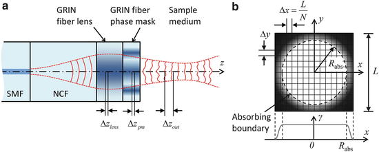
 ![$$ \exp \left(\widehat{N}\Delta z\right)= \exp \left[-i{k}_0\delta n\left(x,y\right)\Delta z\right] $$](/wp-content/uploads/2017/03/A76297_2_En_83_Chapter_IEq15.gif) . For computational efficiency, the diffraction operator is applied in the spatial frequency domain. The simulation geometry is illustrated in Fig. 81.3a. The complex amplitude of the approximately Gaussian beam emitted by the SMF [29] is used as the input field to the BPM simulation, which begins at the NCF/GRIN interface. The field is then numerically propagated through the GRIN fiber lens, through the optional GRIN fiber phase mask, and into the sample medium with BPM step sizes Δz lens , Δz pm , and Δz out , respectively. In the transverse dimensions, the field is sampled on a N × N Cartesian grid of size L. The criteria that govern the appropriate choice of step size Δz and transverse sampling intervals Δx, Δy are discussed in [22]. In order to prevent large-angle diffracted light from reaching the edges of the grid and causing artifacts in the FFT, we apply an “absorbing boundary” (a two-dimensional (2D) window function) to the field amplitude in the spatial domain at every BPM step as illustrated in Fig. 81.3b.
. For computational efficiency, the diffraction operator is applied in the spatial frequency domain. The simulation geometry is illustrated in Fig. 81.3a. The complex amplitude of the approximately Gaussian beam emitted by the SMF [29] is used as the input field to the BPM simulation, which begins at the NCF/GRIN interface. The field is then numerically propagated through the GRIN fiber lens, through the optional GRIN fiber phase mask, and into the sample medium with BPM step sizes Δz lens , Δz pm , and Δz out , respectively. In the transverse dimensions, the field is sampled on a N × N Cartesian grid of size L. The criteria that govern the appropriate choice of step size Δz and transverse sampling intervals Δx, Δy are discussed in [22]. In order to prevent large-angle diffracted light from reaching the edges of the grid and causing artifacts in the FFT, we apply an “absorbing boundary” (a two-dimensional (2D) window function) to the field amplitude in the spatial domain at every BPM step as illustrated in Fig. 81.3b.
:(81.4)
and k 0 denotes the propagation constant in vacuum. In optical fibers, the refractive index variation is on the order of a few percent, and therefore, the refractive index can be expressed as , where is a constant background refractive index (e.g., the index of the silica cladding) and δn(x, y) is a small transverse index variation. The scalar field amplitude can be written as , where is the propagation constant in the background medium and is a complex wave amplitude. For small axial step sizes Δz, an approximate solution to Eq. 81.4 can be written in operator notation:(81.5)
is the diffraction operator in a homogeneous medium with the background refractive index and is an operator which accounts for the inhomogeneity of the refractive index. We can therefore approximate the propagation in the inhomogeneous medium as a repeated cycle of free-space propagation in a thin slice of homogeneous material of thickness Δz and multiplication of the wavefront with a phase screen . For computational efficiency, the diffraction operator is applied in the spatial frequency domain. The simulation geometry is illustrated in Fig. 81.3a. The complex amplitude of the approximately Gaussian beam emitted by the SMF [29] is used as the input field to the BPM simulation, which begins at the NCF/GRIN interface. The field is then numerically propagated through the GRIN fiber lens, through the optional GRIN fiber phase mask, and into the sample medium with BPM step sizes Δz lens , Δz pm , and Δz out , respectively. In the transverse dimensions, the field is sampled on a N × N Cartesian grid of size L. The criteria that govern the appropriate choice of step size Δz and transverse sampling intervals Δx, Δy are discussed in [22]. In order to prevent large-angle diffracted light from reaching the edges of the grid and causing artifacts in the FFT, we apply an “absorbing boundary” (a two-dimensional (2D) window function) to the field amplitude in the spatial domain at every BPM step as illustrated in Fig. 81.3b.Fig. 81.3
(a) Schematic of the BPM simulation geometry for a fiber-optic probe. SMF single-mode fiber, NCF no-core fiber. (b) The N × N simulation grid with size L and with an absorbing boundary of radius R abs (Figure adapted from [22])
One of the main motivations for using the BPM to simulate fiber-optic probes is that it allows the modeling of realistic GRIN fiber lenses [22]. While the ABCD matrix of a GRIN lens is a highly idealized model representing a perfect square-law medium of infinite transverse extent, the refractive index profiles of real GRIN fibers differ from this ideal in a number of ways, as illustrated in Fig. 81.4a. Firstly, the profile is never a perfect parabola, but it is described by a power-law profile that is truncated at the core radius a of the multimode fiber (MMF):
![$$ n(r)=\left\{\begin{array}{cc}\hfill {n}_1{\left[1-2\Delta {\left(\frac{r}{a}\right)}^{\alpha}\right]}^{1/2}\hfill & \hfill r<a\hfill \\ {}\hfill {n}_2={n}_1{\left(1-2\Delta \right)}^{1/2}\hfill & \hfill r\ge a\hfill \end{array}\right. $$](/wp-content/uploads/2017/03/A76297_2_En_83_Chapter_Equ6.gif)
where Δ = (n 12 − n 22)/2n 12 is the relative index difference between the core and cladding refractive indices n 1 and n 2 (for small index differences, Δ ≅ Δn/n 1, where Δn = n 1 − n 2). The influence of the power-law exponent α on the profile shape is indicated in Fig. 81.4b. Secondly, the profiles of GRIN fibers fabricated using the modified chemical vapor deposition (MCVD) method exhibit a characteristic central index dip as well as ripples, where the dip results from “burn-off” of dopant during the high-temperature collapse of the preform, and the ripples result from the deposition of a finite number of layers of changing composition in order to approximate the desired power-law shape [38]. Improved preform fabrication methods [14, 39] have led to a new generation of high-bandwidth GRIN MMFs with smooth refractive index profiles which are free of the central index dip that plagues legacy GRIN MMFs. However, these modern high-bandwidth GRIN MMFs are only available with small core diameters of 50 and 62.5 μm, limiting their use to probe designs with relatively low numerical aperture (NA) and short working distance (WD). Furthermore, their index profiles tend to exhibit a more or less pronounced deviation from the ideal parabolic shape that is purposely introduced by the manufacturer in order to minimize pulse broadening in the targeted operating wavelength band [40–42]. Thus, large core-diameter fibers drawn from preforms of such high-bandwidth GRIN MMFs [14] will not necessarily behave as ideal GRIN lenses.
Fig. 81.4
(a) Power-law refractive index profile with central dip and ripple. (b) Effect of the power-law exponent α on the profile shape. (c, d) Measured index profiles and power-law fits of commercial GRIN multimode fibers (the cladding index n 2 is set to the refractive index n = 1.453 of pure silica at 800 nm). (c) 100-μm core-diameter GRIN MMF (100/140 MMF, POFC, Taiwan). (d) 62.5-μm core-diameter GRIN MMF (GIF625, Thorlabs, USA) (Figure adapted from [22])
(81.6)
Two example index profiles of commercial GRIN fibers together with their best-fit power-law profiles are shown in Fig. 81.4c and d. Figure 81.4c shows a 100-μm-core-diameter GRIN MMF (100/140 MMF, POFC, Taiwan) which was profiled on an EXFO NR-9200 fiber analyzer at a wavelength of 655 nm. The fiber has an α parameter of 2.1 and a central index dip. We have observed that fiber probes made using this GRIN fiber exhibit significant beam distortions that can be reproduced in BPM simulations [22]. Figure 81.4d shows a 62.5-μm-core-diameter GRIN MMF (GIF625, Thorlabs, USA) which we have used extensively in recent work [16, 11, 43, 32] because probes fabricated using this fiber have exhibited very good Gaussian-like beam quality and shown fairly good agreement with ABCD matrix calculations. This observation is not surprising when one considers the index profile (data provided by Thorlabs), which has a near-parabolic shape with an α parameter of 1.96 and no measurable dip in the center.
A deviation of the refractive index profile from the ideal parabolic shape in a GRIN lens is equivalent to spherical aberration (SA) in a refractive lens, with α > 2 producing positive SA and α < 2 producing negative SA [22]. This can be seen in Figs. 81.5a and b, which show BPM simulation results of lensed fibers with power-law GRIN profiles that have α parameters of 2.15 and 1.85, respectively (these values are representative of the maximum deviations from the ideal which one may encounter in real GRIN MMFs). The simulated probes consist of SMF with a mode-field diameter of 5 μm at an operating wavelength of 800 nm, with a 275-μm-long section of NCF and a 280-μm-long section of GRIN MMF with a core diameter of 100 μm, Δ = 2 %, and cladding index n 2 = 1.453. For an aberration-free GRIN fiber with α = 2.0 (or a gradient parameter  ), an ABCD matrix simulation yields an ideal Gaussian output beam with a working distance of 390 μm and a 1/e2 focal spot diameter of 8.5 μm (FWHM diameter of 5 μm), which is shown for comparison by the dotted curves in the plots of Figs. 81.5a and b (bottom). When the α-parameter of the index profile is “de-tuned” to a value of 2.15 (causing a deformation of the profile shape which is just barely noticeable compared to the ideal parabolic curve in Fig. 81.5a (top)), the focal region takes on an asymmetric shape characteristic of spherical aberration. The focal spot intensity is reduced with a Strehl ratio of S = 0.77, while the DOF remains approximately the same as in the aberration-free case. When the α parameter is de-tuned to 1.85, however, the output beam DOF is increased by a factor 1.44 at the cost of only a very slightly reduced Strehl ratio of S = 0.96, showing that GRIN profiles with α < 2.0 can potentially be used to enhance the DOF of fiber probes.
), an ABCD matrix simulation yields an ideal Gaussian output beam with a working distance of 390 μm and a 1/e2 focal spot diameter of 8.5 μm (FWHM diameter of 5 μm), which is shown for comparison by the dotted curves in the plots of Figs. 81.5a and b (bottom). When the α-parameter of the index profile is “de-tuned” to a value of 2.15 (causing a deformation of the profile shape which is just barely noticeable compared to the ideal parabolic curve in Fig. 81.5a (top)), the focal region takes on an asymmetric shape characteristic of spherical aberration. The focal spot intensity is reduced with a Strehl ratio of S = 0.77, while the DOF remains approximately the same as in the aberration-free case. When the α parameter is de-tuned to 1.85, however, the output beam DOF is increased by a factor 1.44 at the cost of only a very slightly reduced Strehl ratio of S = 0.96, showing that GRIN profiles with α < 2.0 can potentially be used to enhance the DOF of fiber probes.Fig. 81.5
BPM simulation results of lensed fiber probes using GRIN fiber lenses that have nonparabolic refractive index profiles with α parameters of 2.15 (a) and 1.85 (b). Top: refractive index profile of the GRIN fiber compared to an ideal parabolic profile with α = 2.0. Middle: simulated E-field amplitude in the entire simulated region. Bottom: FWHM beam diameter and on-axis intensity of the simulated output beam (solid lines) compared to the ideal Gaussian beam that would result in the case of a parabolic profile (dotted lines) (Figure adapted from Ref. [22])
Using the BPM, we have also investigated the effects of the central index dip and index ripple on the output beam [22]. The results indicate that the detrimental effects of such anomalies in the index profile are not as serious as one might expect. This can be understood when one recognizes that the dip and the index ripple are aberrations with high spatial frequencies that generate large-angle diffracted waves which, for parameters that are representative of realistic index profiles, carry only a small percentage of the incident beam power and rapidly lose intensity as they propagate away from the probe end due to their strong divergence. By contrast, the majority of the incident beam power remains in an essentially unperturbed component of the wavefront which converges normally to form an almost unaltered focal region with only a minor reduction in Strehl ratio and no significant change in DOF. This is in stark contrast to index profile aberrations with low spatial frequencies, such as nonideal α parameters or systematic deviations from the power-law model, which will have a strong influence on the intensity distribution in the focal region even for very small index profile errors on the order of a few percent [22]. This finding is important for specifying the fabrication tolerances of customized preforms for high-quality GRIN fiber lenses.
Our results show that the BPM enables accurate simulation of fiber probes using a realistic model of the refractive index profile of the GRIN fiber, which is important in the design of high-performance miniaturized fiber-optic probes for OCT. Furthermore, in Sect. 81.2.4.4, we will demonstrate the use of the BPM for studying schemes for extending the DOF of miniaturized fiber probes using GRIN fiber phase masks.
81.2.2 Scan Mechanisms
OCT imaging, in the sense that 2D or 3D structural information is obtained, is only possible if the probe beam can be scanned within the sample. In the following, we will give a categorization of scanning probes, based on mechanical and optical principles, which is independent of the technical details of the scan mechanism implementation. This categorization will allow us to gain some insight into the advantages and disadvantages of different classes of currently employed scan mechanisms, and it is general enough to accommodate future developments.
Firstly, probes can be categorized into forward-facing and side-facing types (see Fig. 81.6). Generally, the requirements of the application dictate which of these two is preferable.
Fig. 81.6
Side-facing (a) and forward-facing (b) probes. The indicated beam scanning motions in (a) and (b) are just examples, and a variety of other possibilities exist in both cases
Furthermore, probes can be categorized according to their scan mechanisms. There are two main categories of scan mechanisms: beam scanning and probe scanning. The two categories and some of their variations are illustrated in Fig. 81.7. Beam scanning involves a movement of the beam path inside the probe housing, allowing the probe to remain stationary during the scan. Probe scanning, on the other hand, mechanically actuates the entire probe (or a mechanical subcomponent thereof which defines the emitting beam aperture), while the beam path inside the probe is unchanged. Beam scanning probes are more challenging to miniaturize, as they usually require moving parts inside the probe housing. For this reason, probes with submillimeter dimensions generally utilize probe scanning.
Fig. 81.7
Overview of some basic scan mechanisms, categorized into “beam scanning” and “probe scanning”. (a) Image-space scanning (using an oscillating fiber tip in this example). (b) Pupil scanning. The dashed grey rectangle represents a beam deflection mechanism, which can be implemented using various technologies – see text for practical examples. (c) Object-space scanning. (d) Rotation/pullback scanning. (e) Linear-scanning probe inside an outer housing
In beam scanning, the moving beam is projected out of the probe housing into the sample by the probe optics. The probe optics form an imaging system which images scattered light from the sample (the object) onto the sample-arm fiber tip (the image). Using terminology from imaging optics, we can further subdivide beam scanning techniques as “image-space scanning” (Fig. 81.7a), “pupil scanning” (Fig. 81.7b), or “object-space scanning” (Fig. 81.7c). Although Fig. 81.7a, b shows forward-facing configurations for pupil and image-space scanning, they can in principle also be realized as side-facing types by adding mirrors or prisms to deflect the beam outward at a chosen angle.
Image-space scanning (Fig. 81.7a) can be performed by actuating the tip of the sample-arm fiber. The probe beam focal spot is thereby scanned in the sample over a range, which is determined by the magnification of the probe optics. The concept of image-space scanning has been implemented in endoscopic probe designs using oscillating fiber tips [44], but the miniaturization of these designs to submillimeter diameters has proven to be challenging. Small-diameter forward-facing OCT probes of this type have been reported with outer diameters (ODs) of 2.4 and 2.2 mm using tubular four-quadrant piezoelectric actuators [45] and electrostatic actuators [46], respectively.
Pupil scanning (Fig. 81.7b) involves an angular deflection of the collimated beam in the pupil plane of the imaging optics. This is the principle of conventional beam scanning solutions based on galvanometer mirrors, which are positioned in the back focal plane of the scan lens. Beam deflection mechanisms for pupil-scanning probes have been realized with MEMS mirrors [47] and with counterrotating wedged GRIN lens pairs (paired-angle-rotation scanning, PARS [48]). In pupil-scanning arrangements, MEMS mirror solutions require a folded beam path geometry, resulting in relatively large probe diameters of several millimeters. However, PARS probes have been miniaturized to needle dimensions as small as 21 gauge (21G, OD 0.82 mm) in a forward-facing configuration [7].
Object-space scanning (Fig. 81.7c) sacrifices some of the working distance of the probe optics, but is often used in side-facing miniaturized MEMS mirror probes [49, 50] because the MEMS mirror can conveniently serve as the output beam deflector, which directs the beam sideways out of the probe. Although probes of this type with diameters down to 2.6 mm have been demonstrated [50], MEMS technology does not yet seem to allow miniaturization to submillimeter dimensions at the time of writing and is, therefore, mainly targeted toward endoscopic OCT applications.
An elegant variation of beam scanning involves the use of long and thin GRIN relay rods, which can be inserted into hypodermic needles. By scanning the incident light at the proximal end face of the GRIN relay rod, the relayed and focused beam is scanned in object space at the distal end of the relay. The key advantage of this approach is that the scan mechanism does not need to be miniaturized to the diameter of the needle and can be relocated into a larger-diameter housing to which the needle is attached. Submillimeter diameter needle probes of this kind have been demonstrated for multiphoton and confocal endomicroscopy [51, 52] and OCT [53]. In these needle probes, the GRIN relay rod is an integral part of the distal focusing optics. Depending on the scanning mechanism at the proximal end face of the relay (e.g., by scanning the sample-arm fiber tip [52] or scanning an image of it using a galvanometer mirror and objective lens [53]), they can be classified as either image-space or pupil-scanning types, respectively.
In order to achieve the highest possible degree of miniaturization, probe-scanning techniques (Fig. 81.7d, e) must be used, with the smallest reported probe of this kind being encased in a 30G needle (0.31 mm OD) [16]. Probe-scanning designs must be side facing in order to enable at least 2D scanning capability. The most widespread approach is the rotation/pullback method of Fig. 81.7d, where B-scans are acquired over one probe rotation and then stacked along the translation direction to generate a 3D image in a similar fashion to endoscopy [20]. An alternative is to perform a fast translation along the probe axis to acquire a 2D image, as illustrated in Fig. 81.7e, and needle probes of this design have been employed in applications that require a fast 2D scan in a plane parallel to the needle axis, such as dynamic imaging of alveoli [5] and Doppler imaging [12, 54].
An interesting new development in the area of probe scanning is to use freehand motion to scan over a region of interest [55, 8, 56]. This approach can be combined with methods to correct for the resulting nonuniformity of the scan motion as well as the misalignment of adjacent A-lines in the OCT image data, either by using feedback control to actively compensate the probe position during the scan [55] or by post-processing of the OCT image data in combination with location data from a position sensor [56].
81.2.3 A Review of Published Needle Probe Designs
In the following subsections, we will give an overview of the technical evolution of OCT needle probes that are capable of acquiring 2D or 3D images via some form of scanning, as described in Sect. 81.2.2. The term “imaging needle,” which was coined in [2], is useful because it differentiates such scanning needle designs from “point-sensing” fiber probes that are integrated into needles, typically in a forward-facing configuration. Point-sensing needles measure 1D structural information from A-scans acquired at a stationary position or during needle advancement, and a number of examples have been reported. Sequences of A-scans (M-mode) acquired during needle advancement can be displayed as 2D arrays of depth versus time that allow the successive penetration of tissue layers to be visualized [57] (see also Sect. 81.3.1.2). Alternatively, the relative displacement of scatterers in consecutive A-scans can be analyzed in order to determine the mechanical properties of soft tissue that lies ahead of the needle [58]. Processing of single A-scans acquired with point-sensing needles has been used to obtain localized tissue parameters such as the refractive index [59, 60] or attenuation coefficient [4]. An exhaustive discussion of the technology and applications of point-sensing needles lies outside the scope of this section, and we will, therefore, focus our attention on imaging needles.
81.2.3.1 Side-Facing Rotation/Pullback Imaging Needles
The first demonstrated OCT imaging needle probe [2] was a side-facing design for 2D rotation scanning (see Fig. 81.8a). Even though the distal focusing optics used discrete micro-optical components (a 250-μm diameter GRIN lens and a micro-mirror), it already achieved very compact dimensions with an OD of only 0.41 mm (27G). The use of discrete micro-optics introduces challenges related to precision alignment of components inside the needle shaft, and it requires angled or antireflection-coated interfaces in order to avoid backreflections which can introduce image artifacts and reduce the sensitivity. For this reason, many subsequent probe designs were based on “monolithic” all-fiber distal focusing optics using fusion-spliced GRIN fiber lenses or fused ball lenses. The great advantage of such all-fiber probe designs is that they can be fabricated using established fusion splicing technology, which is reproducible and self-aligning. Furthermore, the fusion-spliced optics assembly practically eliminates backreflections from optical interfaces.
Fig. 81.8
Side-facing needle designs for rotation/pullback scanning. (a) The first demonstrated OCT imaging needle probe [2]. (b) The first needle probe to generate full 3D OCT data sets using rotation/pullback scanning [61]. (c) A capillary-encased design with a robust optical-quality output window that can be flat polished for elimination of astigmatism [17]. (d) A catheter-based needle probe for biopsy guidance in lungs [6]. (e) The smallest demonstrated OCT imaging needle probe [16]. (f) A fully fused capillary-encased needle design capillary-encased needle design with an astigmatism-free output beam and with the highest reported sensitivity [11]
Figure 81.8b shows an example of such a design, which was the first OCT needle probe to demonstrate full 3D imaging using combined rotation and pullback [61]. A 23G (0.64 mm OD) side-facing probe was made using a GRIN-lensed fiber which was embedded together with a side-deflecting mirror in UV-curing optical adhesive. Due to the relatively high refractive index contrast between the GRIN fiber end face and the optical adhesive, this interface can be conveniently employed as the reference reflector in a common-path OCT configuration, as was done in Refs. [61, 3, 43]. A drawback of this design is the lack of mechanical robustness of the optical adhesive surface that forms the interface with the sample medium. Mechanical and chemical wear can degrade the optical quality of this interface, leading to deterioration in the sensitivity and beam quality after prolonged use. Furthermore, the shape of the optical adhesive surface cannot be exactly controlled, leading to some distortion and astigmatism in the output beam [43]. An improved needle probe design with an OD of 0.51 mm (25G) using a flat-polished capillary output window has been demonstrated to address this problem [17] (see Fig. 81.8c). By using index-matching fluid inside the capillary, it was shown that the astigmatism could be almost completely eliminated in this design, and the glass capillary provides a robust optical-quality output window interface, at the cost of a more complex fabrication and assembly process.
An example of an all-fiber probe using a fused ball lens is shown in Fig. 81.8d [6]. This 21G (0.82-mm OD) design uses a polyimide catheter to encase the fiber probe, in order to maintain the refractive power of the ball lens in air and to serve as a protective sheath that allows rotation/pullback scanning of the probe while keeping the needle and catheter stationary. The astigmatism which is introduced by the catheter was partially compensated by the shape of the ball lens, which has different radii of curvature in the sagittal and tangential planes.
Ultrathin needle probes with a diameter of only 0.31 mm (30G) were presented in [16] and [32]. These probes use an all-fiber distal optics design that was initially proposed in a patent covering a variety of ultrathin fiber probes for endoscopy [62], where an angle-polished NCF section that is added after the GRIN lens section is used as the side-deflecting mirror as shown in Fig. 81.8e. The angle-polished probe tip is coated with gold in order to maintain its reflectivity under immersion in fluids. A drawback of this probe design is the astigmatism which the beam acquires as it exits from the side of the fiber cladding, which behaves as a cylindrical lens. However, it was shown in [16] and [32] that the astigmatism is reduced to a tolerable level under the near-index-matched conditions existing when the probe is inserted into tissue. This probe design and some of its recent improvements will be presented in more detail in Sect. 81.2.4.2. A needle-like catheter probe incorporating a similar angle-polished GRIN-lensed fiber was presented in [9] for imaging of brain tissue. The 360-μm OD catheter was delivered via a 24G (0.57-mm OD) needle, and the astigmatism of the probe was compensated using index-matching fluid inside the catheter.
An advanced 23G (0.64-mm OD) needle probe design which uses an angle-polished fiber under total internal reflection (TIR) is shown in Fig. 81.8f [11]. The TIR is maintained under fluid immersion by encasing the angle-polished fiber probe inside a microcapillary which is collapsed and fused onto the fiber. The capillary acts as a robust, well-defined optical window, and its astigmatism is compensated using a novel optical design that exploits the focal shift effect [11]. This design achieved the highest reported sensitivity for an OCT needle probe (112 dB) and will be discussed in more detail in Sect. 81.2.4.1.
81.2.3.2 Side-Facing Linear-Scanning Imaging Needles
In contrast to rotation/pullback scanning which combines a fast rotation with a slow linear motion in order to acquire a 3D cylindrical volume, linear-scanning needle probes perform a rapid linear motion along the needle axis in order to generate fast 2D image frames. This can be advantageous for applications where a fast update rate of a large rectangular 2D field of view (FOV) is desirable.
The first linear-scanning OCT needle probes were developed for Doppler imaging and are shown in Fig. 81.9a, b [12]. Two versions were demonstrated, one with an angle-polished GRIN lens and one with an angle-polished ball lens. In both cases, TIR at the angle-polished interface was ensured by sealing the side opening in the 19G (1.1-mm OD) needle with a flat plastic window. These probes allowed imaging at a rate of 1–2 Hz over a linear scan range of ∼2.5 mm. In a later version [54], the dimensions of the probe were reduced by using all-fiber probe optics consisting of GRIN fiber and an angle-polished NCF tip section that were enclosed in a protective catheter that was delivered via a 22G (0.72-mm OD) needle as illustrated in Fig. 81.9c.
Another application which requires a fast 2D frame rate over a large FOV is dynamic imaging of lungs, where a 1.27-mm OD (18-G) linear-scanning needle probe was demonstrated [5] (see Fig. 81.9d and also Sect. 81.4.2.3). An inner side-facing needle probe with a similar design to the one shown in Fig. 81.8b was actuated inside the outer 18G needle at a rate of 3 Hz over a linear scan range of ∼12 mm.
81.2.3.3 Forward-Facing Imaging Needles
The mechanical requirements of a sharp needle tip for easy tissue penetration are not straightforward to combine with the optical requirements of a forward-facing imaging system. For this reason, forward-facing imaging needle probes are typically only used for special applications where a blunt front end is acceptable or even desirable.
A forward-facing OCT needle probe concept called paired-angle-rotation scanning (PARS) [48, 7] has been developed for aiding specialized surgical procedures in the eye. As illustrated in Fig. 81.10a, two angled GRIN lenses are mounted in an inner and an outer needle that rotate in opposite directions, causing the output beam to perform a fanlike sweep back and forth on a line trajectory ahead of the needle. The smallest demonstrated probe of this type had an OD of 0.82 mm (21G) [7].
Another application which requires needlelike forward-facing OCT probes is interventional guidance in neurosurgery. Figure 81.10b shows a 0.74-mm OD (slightly larger than 22G) forward-facing needle incorporating a 0.5-mm-diameter, 12-cm-long GRIN relay rod that was proposed for this application [53]. The input beam to the GRIN relay rod was scanned using galvanometer mirrors that were incorporated into a prototype handpiece attached to the needle. The FOV of this probe was a circular region of 0.44-mm diameter, limited by the diameter of the GRIN relay rod. As an alternative to this approach, somewhat larger, forward-facing needle-like probes with outer diameters of ∼2 mm have been developed that employ an electrostatically actuated oscillating fiber tip inside the needle shaft [46, 10].
81.2.4 Advanced Needle Probe Designs
81.2.4.1 High-Sensitivity Anastigmatic Imaging Needles
OCT needle imaging systems must achieve optical performance comparable to high-end benchtop systems in order to deliver the image quality that is required for clinical applications. The main source of degraded performance in current side-facing OCT needle probes lies in the optics required for deflecting the beam perpendicular to the needle axis, as they tend to introduce losses and beam distortion. We have recently presented a high-optical-quality OCT needle probe that achieves sensitivity and resolution comparable to conventional free-space OCT sample arms [11]. The probe achieves very low optical losses by utilizing total internal reflection (TIR) from an angle-polished fiber tip, encased in a glass microcapillary, as shown in Figs. 81.11a and b. Fusion of the capillary to the fiber provides a robust, optical-quality output window that minimizes beam distortion. Furthermore, the probe features a novel anastigmatic design, which exploits the “focal shift” phenomenon for focused Gaussian beams to achieve equal working distances (WDs) for both axes.
Fig. 81.11
(a) Schematic of the anastigmatic TIR imaging needle design. (b) Bright-field image of the angle-polished fiber probe encased in a fused glass microcapillary. (c) Photo of the fully assembled side-viewing 23G needle (Figure adapted from Ref. [11])
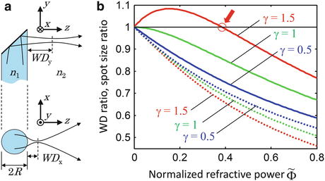
The anastigmatic design concept can be conveniently analyzed using ABCD matrices [27]. As was outlined in Sect. 81.2.1.2, the Gaussian beams transformed using this formalism are exact wave-optic solutions in the paraxial regime and, therefore, intrinsically exhibit the focal shift which is observed when focusing at low Fresnel numbers [63, 27]. Consider a side-facing probe with a cylindrical output window with radius R as shown in Fig. 81.12a. The refractive indices of the cylindrical output window and the sample are n 1 and n 2, respectively. When the initially circularly symmetric beam is deflected sideways out of the probe, its symmetry is broken by the cylindrical interface with refractive power Φ = (n 2 − n 1)/R that acts only in the x-axis (we use a sign convention where the radius R is negative for a concave surface, yielding a positive refractive power for n 2 < n 1). The output beam therefore becomes astigmatic, with WDs and focal spot diameters that will generally be different in the x– and y-axes, as illustrated in Fig. 81.12a. Directly after the cylindrical interface, the complex output beam parameter [27] in the y-direction is equal to
where the minus sign is included to account for the fact that the working distance is a positive number. Inside the probe, directly at the input to the cylindrical interface, the complex beam parameter of the circularly symmetric beam is  . The beam parameter of the output beam in the x-direction is obtained by transforming this beam with the ABCD matrix of the curved interface:
Fig. 81.12
(a) Schematic of a side-viewing probe with astigmatism resulting from the curved output window interface. n1, n2, refractive indices of output window and sample, respectively; WDx, WDy: WD in x and y, respectively; and R, radius of curvature of the output interface. (b) Curves illustrating the WD ratio and spot size ratio as a function of the normalized refractive power, obtained by evaluating Eqs. 81.10 and 81.11 for different values of γ. Solid curves, WD ratio; dotted curves, spot size ratio. The arrow indicates the anastigmatic point (Figure adapted from Ref. [11])
(81.7)
. The beam parameter of the output beam in the x-direction is obtained by transforming this beam with the ABCD matrix of the curved interface:(81.8)
If we introduce the dimensionless variables  and γ = z Ry /WD y , we can write the right-hand side of Eq. 81.8 as
![$$ {\tilde{q}}_{2x}=\frac{-W{D}_y}{{\left(1+\tilde{\Phi}\right)}^2+{\gamma}^2{\tilde{\Phi}}^2}\left[\tilde{\Phi}\left(1+{\gamma}^2\right)+1-i\gamma \right]. $$](/wp-content/uploads/2017/03/A76297_2_En_83_Chapter_Equ9.gif)
and γ = z Ry /WD y , we can write the right-hand side of Eq. 81.8 as(81.9)
After comparing the real and imaginary parts with  , one obtains the following two dimensionless expressions for the ratios of the WDs and spot sizes in the x– and y-directions [11]:
, one obtains the following two dimensionless expressions for the ratios of the WDs and spot sizes in the x– and y-directions [11]:(81.10)
(81.11)
The two ratios given by Eqs. 81.10 and 81.11 are plotted in Fig. 81.12b as a function of the normalized refractive power  for different values of the parameter γ. The curves in Fig. 81.12b can be interpreted as the result of a thought experiment in which a Gaussian beam is transmitted through an initially planar interface between media with the refractive indices n 1 and n 2, coming to a focus with Rayleigh range z Ry at a working distance WD y (thereby determining the parameter γ). One can then imagine increasing the normalized refractive power
  by “bending” the interface in the x-direction. While the y-direction is unaffected, the WD and focal spot radius of the x-direction begin to deviate from WD y and w 0y with increasing refractive power. For beams with γ > 1, the WD of the x-direction initially increases and then decreases again, going through an anastigmatic point where the WDs of the two axes are equal (red arrow in Fig. 81.12b).
for different values of the parameter γ. The curves in Fig. 81.12b can be interpreted as the result of a thought experiment in which a Gaussian beam is transmitted through an initially planar interface between media with the refractive indices n 1 and n 2, coming to a focus with Rayleigh range z Ry at a working distance WD y (thereby determining the parameter γ). One can then imagine increasing the normalized refractive power by “bending” the interface in the x-direction. While the y-direction is unaffected, the WD and focal spot radius of the x-direction begin to deviate from WD y and w 0y with increasing refractive power. For beams with γ > 1, the WD of the x-direction initially increases and then decreases again, going through an anastigmatic point where the WDs of the two axes are equal (red arrow in Fig. 81.12b).Stay updated, free articles. Join our Telegram channel

Full access? Get Clinical Tree


