(32.1)
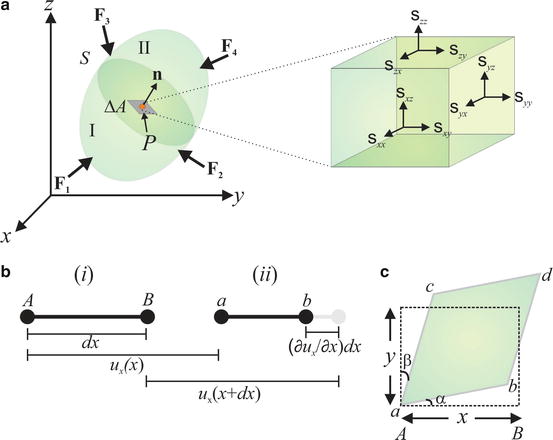
Fig. 32.1
(a) Stress components acting at the point P located within a deformable body under load. (b) Normal strain along the x-axis of the cube in (a) (i) before and (ii) after compressive deformation. The gray line in (ii) represents the initial length. (c) Shear strain: xy-plane of the cube in (a) after shear deformation. The dashed rectangle represents the xy-plane before deformation
The S.I. unit of stress is the Pascal, equivalent to Nm −2. Equation 32.1 defines the particular case where the direction of the resultant force, ΔF, is also the direction of the stress vector. More generally, the direction of the stress vector is inclined to ΔA and is described by two components: a normal stress perpendicular to ΔA and a shear stress acting in the plane of ΔA. Consider the infinitesimal cubic element located at the point P, shown in Fig. 32.1a, with faces parallel to the coordinate axes. Each component of stress acting on the cube is highlighted in Fig. 32.1a. Two subscripts are used for each component. The first indicates the direction of the normal to the plane and the second indicates the direction of the stress component. The total stress acting on the cube is described by a second-order tensor:
![$$ \boldsymbol{\sigma} =\left[\begin{array}{ccc}\hfill {\sigma}_{xx}\hfill & \hfill {\sigma}_{xy}\hfill & \hfill {\sigma}_{xz}\hfill \\ {}\hfill {\sigma}_{yx}\hfill & \hfill {\sigma}_{yy}\hfill & \hfill {\sigma}_{yz}\hfill \\ {}\hfill {\sigma}_{xz}\hfill & \hfill {\sigma}_{yz}\hfill & \hfill {\sigma}_{zz}\hfill \end{array}\right]. $$](/wp-content/uploads/2017/03/A76297_2_En_33_Chapter_Equ2.gif)
(32.2)
32.2.2 Strain Tensor
The strain tensor describes each component of the deformation resulting from an applied load. Consider the x-axis of the infinitesimal cube presented in Fig. 32.1a. In Fig. 32.1b, this axis is shown (i) before and (ii) after compressive deformation. The component u x describes the displacement at the point A. The initial length along the x-axis, ∣AB∣, is given by dx. After deformation, this length (∣ab∣ in Fig. 32.1b) is given by  . The normal strain is defined as the unit elongation/contraction:
. The normal strain is defined as the unit elongation/contraction:(32.3)
The same analysis holds for the normal strain in the y– and z-axes, ε yy and ε zz , defined as  and
and  , respectively. In OCE, the strain defined in Eq. 32.3 is often referred to as the local strain [19]. As the strain is a ratio of lengths, it is dimensionless. By convention, tensile strains are positive and compressive strains are negative. Following this convention, the quantity
  in Fig. 32.1b is negative, and therefore, the compressive strain ε xx is also negative. Analogously to stress, the strain has both normal and shear components. The xy-plane of the cube in Fig. 32.1a is illustrated in Fig. 32.1c. After deformation, the area dxdy takes the form of a parallelogram in the general case. The shear strain is defined as the change in angle between two axes that were originally orthogonal. From Fig. 32.1c, the shear strain, ε xy , is given by α + β. For small displacement gradients, we have
  and
and  , where u y is the displacement along the y-axis at the point A, allowing the shear strain, ε xy , to be defined as
  . By interchanging x and y and u x and u y , it can be demonstrated that ε xy = ε yx . Shear strain components in the xz and yz planes can be defined in a similar manner. The infinitesimal strain tensor describing each component of strain can then be expressed as
![$$ \varepsilon =\left[\begin{array}{ccc}\hfill {\varepsilon}_{xx}\hfill & \hfill {\varepsilon}_{xy}\hfill & \hfill {\varepsilon}_{xz}\hfill \\ {}\hfill {\varepsilon}_{yx}\hfill & \hfill {\varepsilon}_{yy}\hfill & \hfill {\varepsilon}_{yz}\hfill \\ {}\hfill {\varepsilon}_{zx}\hfill & \hfill {\varepsilon}_{zy}\hfill & \hfill {\varepsilon}_{zz}\hfill \end{array}\right]=\left[\begin{array}{ccc}\hfill \frac{\partial {u}_x}{\partial x}\hfill & \hfill 0.5\left(\frac{\partial {u}_x}{\partial y}+\frac{\partial {u}_y}{\partial x}\right)\hfill & \hfill 0.5\left(\frac{\partial {u}_x}{\partial z}+\frac{\partial {u}_z}{\partial x}\right)\hfill \\ {}\hfill 0.5\left(\frac{\partial {u}_y}{\partial x}+\frac{\partial {u}_x}{\partial y}\right)\hfill & \hfill \frac{\partial {u}_y}{\partial y}\hfill & \hfill 0.5\left(\frac{\partial {u}_y}{\partial z}+\frac{\partial {u}_z}{\partial y}\right)\hfill \\ {}\hfill 0.5\left(\frac{\partial {u}_z}{\partial x}+\frac{\partial {u}_x}{\partial z}\right)\hfill & \hfill 0.5\left(\frac{\partial {u}_z}{\partial y}+\frac{\partial {u}_y}{\partial z}\right)\hfill & \hfill \frac{\partial {u}_z}{\partial z}\hfill \end{array}\right], $$](/wp-content/uploads/2017/03/A76297_2_En_33_Chapter_Equ4.gif)
where the shear components are scaled by 0.5, as ε xy = ε yx , ε xz = ε zx , and ε yz = ε zy . It should also be noted that in dynamic elastography techniques, the strain rate is often measured. Strain rate is defined as the rate of change of strain with time [1] and is easily obtained from the expressions defined in Eq. 32.4.
and , respectively. In OCE, the strain defined in Eq. 32.3 is often referred to as the local strain [19]. As the strain is a ratio of lengths, it is dimensionless. By convention, tensile strains are positive and compressive strains are negative. Following this convention, the quantity in Fig. 32.1b is negative, and therefore, the compressive strain ε xx is also negative. Analogously to stress, the strain has both normal and shear components. The xy-plane of the cube in Fig. 32.1a is illustrated in Fig. 32.1c. After deformation, the area dxdy takes the form of a parallelogram in the general case. The shear strain is defined as the change in angle between two axes that were originally orthogonal. From Fig. 32.1c, the shear strain, ε xy , is given by α + β. For small displacement gradients, we have and , where u y is the displacement along the y-axis at the point A, allowing the shear strain, ε xy , to be defined as . By interchanging x and y and u x and u y , it can be demonstrated that ε xy = ε yx . Shear strain components in the xz and yz planes can be defined in a similar manner. The infinitesimal strain tensor describing each component of strain can then be expressed as(32.4)
32.2.3 Constitutive Equation for a Linearly Elastic Solid
Having defined the load applied to tissue using the stress tensor and the resulting deformation using the strain tensor, a constitutive equation relating the two is used to define tissue elasticity. In elastography, the most commonly used constitutive equation is that of a linearly elastic (or Hookean) solid in which the relationship between stress and strain is linear and strain is independent of the rate at which the load is applied. The constitutive equation for a linearly elastic solid is

where i, j, k, and l define each tensor component. As σ and ε are second-order tensors, C is a fourth-order tensor, consisting of 81 elastic constants, referred to as the elasticity tensor. To simplify the analysis, it is frequently assumed that the elasticity is isotropic, i.e., elasticity can be described without reference to direction. This imposes maximum symmetry on the tensor, reducing the 81 elastic constants to two and resulting in the isotropic linear elastic constitutive equation, defined as
where λ and μ are the elastic constants, also known as the Lamé constants, and δ ij is the Kronecker delta (equal to 1 if i = j and 0 otherwise). As ε is dimensionless, the unit for λ and μ is that of stress, i.e., the Pascal. It should be noted that constitutive equations that more accurately model the nonlinear viscoelastic response of soft tissue to loading have also been proposed [20]. However, their complexity has restricted their use in OCE.
(32.5)
(32.6)
32.2.4 Elastic Properties
A number of descriptors may be derived from the Lamé constants for a material’s elastic properties. In this section, we define these descriptors, namely, Young’s modulus, shear modulus, bulk modulus, and Poisson’s ratio and describe their relevance to OCE.
Young’s modulus, E, characterizes the elasticity of a material subjected to uniaxial stress, i.e., only one normal stress component in Eq. 32.2 is nonzero. Uniaxial stress is generally a good approximation for the loads applied in OCE. For a load acting along z, E is defined as σ zz /ε zz , i.e., the ratio of normal (axial) stress to normal (axial) strain. In terms of the Lamé constants, it is expressed as  . E has the same unit as stress, i.e., the Pascal.
. E has the same unit as stress, i.e., the Pascal.Shear modulus, G, is the ratio of shear stress to shear strain, e.g., σ xz /ε xz . It is equal to the Lamé constant, μ, and its unit is the Pascal.
Bulk modulus, K, is defined as the ratio of hydrostatic pressure, σ, to unit volume change, Δv/v. Hydrostatic pressure describes the situation when all shear stress components are zero and the normal stress components are equal, i.e., σ xx = σ yy = σ zz . K is a measure of the compressibility of a material and defined as  , and its unit is the Pascal. Its unit of measurement is the Pascal.
, and its unit is the Pascal. Its unit of measurement is the Pascal.Poisson’s ratio, ν, is defined as the ratio of the normal strain along the axis of stress to the normal strain in each orthogonal axis. In compression, it is the ratio of elongation per unit breadth to contraction per unit length, e.g., −ε xx /ε zz , where the negative sign results from the division of a tensile normal strain, ε xx , by a compressive normal strain, ε zz . It is defined in terms of the Lamé constants as  . As it is a ratio of two strains, it is dimensionless.
. As it is a ratio of two strains, it is dimensionless.The Lamé constants, Young’s modulus, shear modulus, bulk modulus, and Poisson’s ratio are related. Only two of these parameters are independent for an isotropic, linearly elastic material, and thus, measurement of any two determines the other parameters. For soft tissue, the high water content results in the near conservation of volume upon compression. As a result, the bulk modulus of soft tissue has been reported to vary by less than 15 % from that of water [17]. The incompressibility of soft tissue also results in a Poisson’s ratio of very close to but not exceeding 0.5. As these properties do not vary significantly for soft tissues, the goal of most OCE techniques is to estimate Young’s modulus or shear modulus, which has a much larger dynamic range. These moduli also correspond most closely to what is sensed by manual palpation of the tissue. In soft tissue, it is readily shown that E ≈ 3G, under the assumption that ν ≈ 0.5 [16]. Therefore, Young’s modulus is the most common single property used to characterize tissue elasticity and the most commonly probed property in OCE. The value of Young’s modulus of soft tissues extends from tens of Pascals, in very soft tissues such as adipose [21], to hundreds of kPa to MPa, as in hard tumors [22].
32.2.5 Equations of Motion
In some OCE techniques, as well as in some ultrasound and magnetic resonance elastography techniques, a dynamic (sinusoidal) load is applied to the sample. In this case, inertia must be taken into account. The constitutive equation of motion for a linearly elastic solid is given by Navier’s equation as [16]
where ρ is the density of the tissue and u is the displacement vector. Transverse and longitudinal waves can propagate independently in the material: S (shear) waves and P (pressure) waves, respectively. For shear wave propagation, there is no volume change in the material. The dilatation term (∇ ⋅ u) is therefore zero and Eq. 32.7 becomes
where c s , the shear wave speed, is defined as  . Pressure waves are irrotational, i.e., ∇ × u = 0, allowing u to be written in terms of a potential, ψ, such that u = ∇ψ. The wave equation then becomes
where the P-wave speed, c p , is defined as  .
.
(32.7)
(32.8)
. Pressure waves are irrotational, i.e., ∇ × u = 0, allowing u to be written in terms of a potential, ψ, such that u = ∇ψ. The wave equation then becomes(32.9)
.For soft tissues, the pressure wave speed, typically several thousand m/s, is orders of magnitude faster than the shear wave speed, typically several m/s [18]. The focus in dynamic OCE to date has mainly been to measure elasticity from the shear wave properties [23–26]. There are several reasons for this: firstly, as the P-wave speed depends on variations of the bulk modulus, it has a much lower dynamic range in tissue than S-waves; secondly, the high speed of P-waves makes their detection challenging.
An advantage of dynamic OCE is that it should enable the complex dynamic mechanical response of a sample to be measured, providing information about both its elastic and viscoelastic properties. OCE techniques that have been used to measure viscoelastic properties of tissue are discussed in more detail in Sect. 32.4.4. Dynamic OCE is also potentially more suitable for in vivo measurements, as it enables loading in a frequency range not affected by sample motion, e.g., due to breathing.
32.3 Measuring Displacement in OCE
The accuracy and dynamic range of the displacement measured in response to a load has a major impact on elastogram quality. In this section, we describe three techniques to measure the displacement: speckle tracking, phase-sensitive detection, and use of the Doppler spectrum.
32.3.1 Speckle Tracking
Speckle is the phenomenon of fine-scale, apparently random, fluctuating light and dark intensity present in all coherent imaging systems. In OCT, it is generated by the summation of the multiple backscattered optical wavefields arising from the sub-resolution sample scatterers. The wavefields may be represented as a summation of complex phasors, which determines the intensity and phase of the detected signal. A detailed analysis of OCT speckle can be found elsewhere [27].
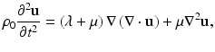
Speckle tracking may be considered to be a sub-branch of the much broader field of speckle metrology, developed since the late 1960s [28, 29]. The utility of speckle for tracking motion in OCE arises because each speckle realization, far from being random, is dependent upon the precise location of backscatterers within the sample. As the backscatterers translate, within a certain range, so does the speckle pattern associated with them. Under the assumption that the relative positions of sub-resolution scatterers remain fixed while they translate, any variation of the speckle pattern between successive acquisitions, or equivalently, of its second-order temporal statistics, can be used to measure sample motion. This is shown in Fig. 32.2, in which a small portion of an OCT speckle pattern acquired from a homogeneously scattering phantom under compressive load (applied from above) is shown in false color. The pattern is shown for four increments in load, increasing from Fig. 32.2a–d. Translation of a single bright speckle is highlighted by a black outline in each figure part. Evident in Fig. 32.2 is the gradual decorrelation of the speckle pattern with load, a major limitation of the technique. This decorrelation is caused by the reorganization of the positions of the sub-resolution scatterers due to loading. It limits the maximum measurable displacement to considerably less than the OCT resolution.
Fig. 32.2
Speckle pattern of a silicone phantom (logarithmic intensity scale) under increasing compressive load (applied from above) from (a–d). Image dimensions 50 × 50 μm. Black outline highlights the evolution of an individual speckle
The speckle shift is typically evaluated by calculating the cross-correlation of a portion of B-scans acquired at two time points during compression [9]. Consider a point scatterer embedded in a transparent medium at position (x, z). When the sample is placed under load, the scatterer is displaced to a new location, (x + Δx, z + Δz). The normalized cross-correlation between the OCT signal before, I 1(x, z), and after loading, I 2(x, z), within a predefined window of dimensions X × Z, is given by
(32.10)
The relative displacement, between the acquisition of I 1(x, z) and I 2(x, z), in the x and z directions can then be determined from
![$$ \Delta {u}_x= \max \left[\left(\rho \left(x^{\prime },z^{\prime}\right)\right)\right]\kern0.5em \mathrm{f}\mathrm{o}\mathrm{r}\kern0.5em z^{\prime }=0,-X/2\le x^{\prime}\le X/2, $$](/wp-content/uploads/2017/03/A76297_2_En_33_Chapter_Equ11.gif)
and
![$$ \Delta {u}_z= \max \left[\left(\rho \left(x^{\prime },z^{\prime}\right)\right)\right]\kern0.5em \mathrm{f}\mathrm{o}\mathrm{r}\ x^{\prime }=0,-Z/2\le z^{\prime}\le Z/2. $$](/wp-content/uploads/2017/03/A76297_2_En_33_Chapter_Equ12.gif)
(32.11)
(32.12)
From Eqs. 32.10–32.12, ρ is maximum for x′ = Δx and z′ = Δz, respectively. Correlation-based speckle tracking was used in early OCE research [9, 30–34] and has been commonly used in ultrasound elastography [3]. Early examples of OCE elastograms obtained using correlation-based speckle tracking, along with the corresponding OCT images, acquired from a Xenopus laevis tadpole at different stages of development are shown in Fig. 32.3.
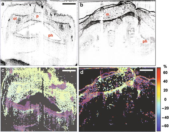
Fig. 32.3
OCT images and strain maps of a Xenopus laevis tadpole at different life cycle stages. (a, c) Representative structural OCT and OCE relative (local) strain maps, respectively, for stage 42 (3 -day-old). (b, d) Representative structural OCT and OCE relative (local) strain maps for Stage 50 (15 -day-old). Scale bar = 300 μm (adapted from [34])
The minimum measurable displacement obtainable with speckle tracking is determined by the spatial sampling in the underlying OCT system, assuming an adequate OCT SNR. For cross-correlation techniques that use a central difference approach to evaluate Eq. 32.10, this corresponds to 0.5 pixels [10]. Displacements as small as 0.1 pixels can be measured using parametric techniques, such as the maximum likelihood estimator [11, 35]. However, these estimators result in intolerably large errors for displacements >0.8 pixels.
The maximum measurable displacement using the cross-correlation method is set by speckle decorrelation, as mentioned, which depends on the sample elasticity as well as on the size range, density, and arrangement of the sub-resolution scatterers. In a study on a silicone phantom containing titanium dioxide particles, the maximum displacement was reported to be ∼0.5 times the resolution of the OCT system [35]. Low OCT SNR also results in decorrelation between successive B-scans [35], reducing the accuracy of displacement measurements with increasing depth in the sample.
The above limits imply a severely limited dynamic range for speckle tracking. Consider an OCT system with spatial resolution of 10 × 10 × 10 μm and spatial sampling such that the axial pixel size is 3 μm and the lateral pixel size is 1 μm. Use of a smaller pixel size either imposes restrictions on the field of view (for fixed pixel count) or increases in the acquisition time (for more pixels). Using cross-correlation, minimum and maximum measurable displacements of ∼1.5 and ∼5 μm (from the example in [36]), respectively, might be reasonably expected and correspond to a dynamic range of ∼3.3, with the same range applying to the measurable elasticity in OCE.
An additional limitation is that the displacement is calculated within a predefined window (X × Z in Eq. 32.10). The window sets the imaging spatial resolution of each displacement measurement, lowering it relative to the OCT image resolution, typically by a factor of 5–10 [9, 31].
An important further consideration when using speckle tracking is the avoidance of decorrelation caused by changes in the tissue configuration not related to its elastic properties, such as bulk motion, Brownian motion, or blood flow. This implies an acquisition speed high enough to ensure the speckles remain correlated between successive scans.
An advantage of speckle tracking is that motion can be tracked in more than one spatial dimension. Speckle tracking in OCE has been performed in only one or two dimensions, but 3D tracking has been proposed in ultrasound [37]. 3D tracking would provide the opportunity to measure shear strain in addition to normal strain (see Eq. 32.4) and to remove the otherwise necessary assumption of isotropic mechanical behavior. This may provide additional OCE contrast in anisotropic tissues, such as skin and muscle, as has already been demonstrated in ultrasound [38] and magnetic resonance elastography [39]. Indeed, 3D information is routinely obtained in magnetic resonance elastography.
32.3.2 Phase-Sensitive Detection
Speckle tracking utilizes changes in the intensity of an OCT image with loading. In Fourier-domain (FD) OCT, after performing a Fourier transform on the detected spectral fringes, the depth-resolved complex signal is obtained. This provides the opportunity to analyze the phase of the detected signal. OCT phase is generally random in soft tissue; however, it is temporally invariant if the sample is stationary. If a sample is subjected to mechanical loading, its axial displacement, Δu z , between two A-scans, acquired from the same lateral position, results in a phase shift, Δϕ [40]. The displacement, Δu z , along the axis of the incident beam is defined as
where λ is the mean wavelength of the source and n is the average refractive index along the beam path. The phase difference is calculated either between two successive A-scans in a B-scan (requiring high lateral sampling density) [40] or between two A-scans acquired in the same lateral position in successive B-scans [41]: the latter is illustrated in Fig. 32.4 with experimental data acquired from a uniformly scattering silicone phantom. Phase-sensitive detection was initially developed for Doppler flow velocity measurement in OCT [42]. Indeed, the phase-sensitive technique is based on the Doppler shift; thus, unlike speckle tracking, only the axial component of the displacement can be detected. If we assume that the maximum measurable displacement is set by the maximum unambiguous phase difference, i.e., 2π, then this corresponds to half the source center wavelength (in the sample medium). The minimum measurable displacement,  , is determined by the phase sensitivity of the OCT system [43], which, in the shot-noise limited regime, is related to the OCT signal-to-noise ratio (SNR) and is approximated as
![$$ {\sigma}_{\Delta \phi }=\frac{1}{\sqrt{SNR}},\kern1em SNR>>1. $$
” src=”/wp-content/uploads/2017/03/A76297_2_En_33_Chapter_Equ14.gif”></DIV></DIV><br />
<DIV class=EquationNumber>(32.14)</DIV></DIV><br />
<DIV id=Fig4 class=Figure><br />
<DIV id=MO4 class=MediaObject><IMG alt=A76297_2_En_33_Fig4_HTML.jpg src=]()
(32.13)
, is determined by the phase sensitivity of the OCT system [43], which, in the shot-noise limited regime, is related to the OCT signal-to-noise ratio (SNR) and is approximated asFig. 32.4
Schematic illustration of phase-sensitive detection with experimental data from a mechanically homogeneous silicone phantom. (a) The phase of OCT B-scans acquired at the same lateral position before (1) and after (2) sample loading. (b) Phase difference between the B-scans shown in (a). As the load was applied from the top, the phase difference is maximum in this position, reducing to near zero at large depths
Park et al., in their work on flow imaging [44], demonstrated good agreement between Eq. 32.14 and experimental results for OCT SNR >30 dB. It is important to emphasize, however, that this approximation is only valid for large OCT SNR.
Another source of phase noise is introduced under the successive A-scans scenario if the temporally displaced beams are not precisely overlapped in space. The phase noise introduced due to lateral beam motion, Δx, between successive A-scans is given by [44]
![$$ {\sigma}_{\Delta x}=\sqrt{\frac{4}{3}\left\{1- \exp \left[-2{\left(\frac{\Delta x}{w}\right)}^2\right]\right\}}, $$](/wp-content/uploads/2017/03/A76297_2_En_33_Chapter_Equ15.gif)
where w is the 1/e 2 beam width at the focus. In practice, to minimize phase noise due to scanning, dense sampling is performed along the axis used to calculate the phase difference. As an example, consider a typical OCT system with a 1/e 2 beam width of 25 μm at the focus. Acquiring A-scans in 1 μm lateral steps ensures that the phase noise due to scanning is <0.05 rad, within a factor of 5 of the limiting phase noise for OCT SNR = 40 dB. A further source of phase noise, σ mech , is introduced by mechanical instabilities in the system, such as jitter in the scanning mirrors. Combining Eqs. 32.14 and 32.15 and including mechanical instabilities, considering each of these processes to be additive and Gaussian, the total phase noise, σ Tot , is given by
(32.15)
(32.16)
To minimize σ Tot , both σΔϕ and σ mech must be negligible and the OCT SNR must be maximized (see Eq. 32.14). Under these conditions, displacement sensitivity of ∼20 pm has been reported [45]. The minimization of σ mech has been discussed in detail in relation to optical coherence microscopy (see Chap. 28, “Optical Coherence Microscopy” for more details). Techniques employed to minimize σ mech include the use of a common-path interferometer and a reference reflector within the sample arm. In practice, σΔϕ is often appreciable due to the requirement to laterally scan across the sample, such that typical displacement sensitivities lie in the range 0.1–1 nm.
A key advantage of phase-sensitive detection over speckle tracking is its larger dynamic range. If we consider the phase difference between two A-scans acquired using an OCT system with mean wavelength of 1300 nm and minimum OCT SNR of 30 dB, the displacement dynamic range in air is >60, almost 20-fold larger than that achievable using the cross-correlation method for speckle tracking described in Sect. 32.3.1.
A major limitation is imposed by phase wrapping, one which invalidates the assumption of a linear relationship between phase difference and displacement (Eq. 32.13). Phase jumps of 2π not only occur when the desired phase difference is close to the 2π limit but also arise due to noise when the OCT SNR is low. In the case of dynamic loading, phase wrapping due to noise can be mitigated by faster acquisition. An alternative means of mitigation is intensity thresholding and weighting, which gives preference to the phase difference estimated from pixels with high SNR. On the other hand, robust algorithms to correctly unwrap phase may enable significant increases in the dynamic range of phase-sensitive OCE, e.g., successfully unwrapping one such event would lead to a 3 dB improvement in dynamic range. However, it must be emphasized that all phase-unwrapping algorithms break down in the presence of high noise.
Phase-sensitive detection possesses several advantages over speckle tracking, including the larger dynamic range, lower computational complexity, and higher displacement sensitivity. Also, the spatial resolution of displacement measurements is matched to that of the underlying OCT system: the displacement is not estimated in an X × Z window, as is the case in speckle tracking.
The above discussion has not explicitly considered determining the displacement by phase measurement under dynamic mechanical loading. Liang et al. [46] developed a technique to measure displacement under dynamic loading using phase-sensitive detection. The vibration amplitude is calculated from the displacement and used to estimate the strain rate. A related technique has also been presented for measuring vibration within the ear [45]. In the next section, we consider a recently introduced improvement over these phase-sensitive methods for detecting vibration amplitude.
32.3.3 Doppler Spectrum
A major limitation of phase-sensitive detection is the large drop-off in accuracy with decreasing SNR (Eq. 32.14). Recently, with the goal of reducing this drop-off, a new technique has been proposed for extracting the displacement from the measured intensity under dynamic mechanical loading. Joint spectral- and time-domain optical coherence elastography (STdOCE) improves vibration amplitude measurement in dynamic OCE [47] by adapting the technique previously proposed for Doppler flow imaging [48]. STdOCE provides more accurate vibration amplitude measurements than the phase-sensitive technique in the case of low OCT SNR (<20 dB), thereby extending the depth range of accurate dynamic OCE measurements.
Dynamic loading results in an amplitude spectrum of frequency tones described by Bessel functions of the first kind. In STdOCE, a Fourier transform is performed in the time domain, i.e., across multiple A-scans. If the A-scan rate is much higher than the loading rate, the result is a Doppler spectrum containing frequency tones, which can be used to extract the vibration amplitude at each depth in the sample.
STdOCE is closely related to a previously reported dynamic OCE technique based solely on time-domain (TD) OCT [19, 49]. The bandwidth of the frequency tones in TD-OCT increases with both the bandwidth of the source and the A-scan velocity, which causes them to overlap in frequency and restricts measurements to only the first few tones. This limits the accuracy and requires the use of a very slow A-scan acquisition rate (∼1 Hz). Nonetheless, this technique was capable of being used to demonstrate the first in vivo dynamic OCE measurements [49].
In STdOCE, the increased number of tones in the Doppler spectrum provided by spectral-domain (SD) OCT allows a signal processing technique proposed in ultrasound elastography to be employed [50], in which the vibration amplitude is determined from the variance or spectral spread of frequency tones in the Doppler spectrum. Figure 32.5 shows the data acquisition and processing procedure for STdOCE. In Fig. 32.5a, 2,000 successive spectral interferograms acquired from the same lateral position in a homogeneous phantom are shown. In Fig. 32.5b, the corresponding depth-resolved A-scans, after Fourier transformation in k-space, are shown. In Fig. 32.5c, the Doppler spectrum obtained after performing a second Fourier transform in the time domain at the depth indicated by the red line in Fig. 32.5b is shown, with nine overtones in evidence. Having calculated the Doppler spectrum, the spectral spread algorithm is used to calculate the vibration amplitude. The vibration amplitude calculated from the spectrum in Fig. 32.5c is indicated by the red dot in Fig. 32.5d. This procedure is repeated for each depth in the sample, allowing a vibration amplitude plot (blue line in Fig. 32.5d) to be generated.
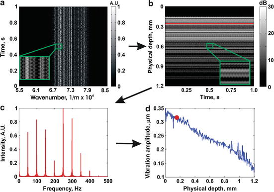
Fig. 32.5
Data processing procedure for STdOCE: (a) 2,000 spectral interferograms; (b) A-scans obtained after Fourier transform in k-space; (c) Doppler spectrum after Fourier transform in time, performed at depth indicated by the red line in (b); and (d) vibration amplitude (peak) calculated using the spectral spread algorithm. The red dot in (d) corresponds to the vibration amplitude calculated from the Doppler spectrum in (c) (reproduced from [47])
Figure 32.6 demonstrates the superiority of STdOCE over a representative technique for phase-sensitive detection [45]. In Fig. 32.6a, a structural OCT image of a soft phantom containing a stiff inclusion is shown. The inclusion is located in the center of the image and is indicated by the labeled arrow. Below the inclusion, a shadow artifact, corresponding to a region of low OCT SNR, is also labeled. A plot of the OCT SNR, at the lateral position indicated by the vertical red arrow in Fig. 32.6a, is shown in Fig. 32.6d. Vibration amplitude images generated using STdOCE and phase-sensitive OCE are shown in Fig. 32.6b, f, respectively. In both images, the stiff inclusions are denoted by the lower rate of change in vibration amplitude with depth, i.e., lower strain. Vibration amplitude plots generated using both techniques, at the lateral position indicated by the red arrow in Fig. 32.6a, are shown in Fig. 32.6e. Both plots match well until a depth of ∼600 μm. At depths >600 μm, the decrease in vibration amplitude is higher for the phase-sensitive technique (red). This is caused by an underestimation of the vibration amplitude in the low OCT SNR region below the inclusion. In comparison, the decrease in vibration amplitude with depth measured with STdOCE below the inclusion is the same as that above the inclusion, as expected for these mechanically uniform regions. The strain elastograms corresponding to Figs. 32.6b and f are shown in Figs. 32.6c and g, respectively. The artificially high strain in the phase-sensitive elastogram (Fig. 32.6g) is clearly visible below the inclusion. As the elastogram is used as a surrogate for elasticity, this leads to errors in the interpretation of elastograms.
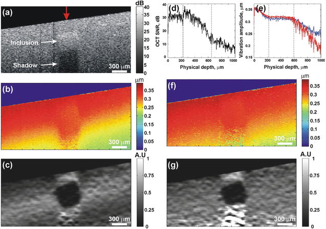
Fig. 32.6
Soft phantom containing a stiff inclusion: (a) OCT structural image; (b) vibration amplitude image; (c) elastogram for STdOCE; (d) OCT A-scan; (e) vibration amplitude plots for STdOCE (blue) and phase-sensitive OCE (red) at the lateral position indicated by the red arrow in (a), where the dashed lines in (d) and (e) indicate the boundaries between the soft bulk and hard inclusion; (f) vibration amplitude image; and (g) elastogram for phase-sensitive OCE [47]
In this section, we described the two main techniques used to measure the displacement in OCE: the technique used in early OCE papers, speckle tracking, and the most commonly used technique in recent papers, phase-sensitive OCE. A recent improvement on phase-sensitive OCE that applies to dynamic displacement, STdOCE, based on the analysis of the Doppler spectrum, was also described. As discussed, each technique has its advantages and disadvantages, and these are summarized in the table below. It is expected that phase-sensitive techniques will continue to be prominent, as they enjoy a significantly larger dynamic range than speckle tracking and require the acquisition of much less data than STdOCE (Table 32.1).
Table 33.1
Comparison of different methods to measure displacement in OCE
Minimum displacement | Maximum displacement | Axial resolution | Lateral resolution | Dimension of elasticity measured | Minimum data required | |
|---|---|---|---|---|---|---|
Speckle tracking | ∼0.1 × pixel size | ∼0.5 × OCT resolution | 5–10 × OCT resolution | 5–10 × OCT resolution | 1D, 2D, 3D | 2 A-scans |
Phase-sensitive | ∼20 pm | ∼0.5 × source wavelength | OCT resolution | OCT resolution | 1D | 2 A-scans |
Doppler spectrum | ∼10 nm | ∼0.5 × OCT axial resolution | OCT resolution | OCT resolution | 1D | >10 A-scans |
32.4 OCE Techniques
In this section, we consider the wide variety of techniques that have been used to estimate elasticity from the measured displacement, as categorized by the nature and dynamics of the loading mechanism. We divide OCE techniques into five categories: compression, surface acoustic wave, acoustic radiation force, magnetomotive, and spectroscopic.
32.4.1 Compression
In compression OCE, a step load is introduced externally to a sample between acquisitions (of either A-scans or B-scans) and the strain is estimated from the change in measured displacement with depth. This technique was used by Schmitt et al. in the first demonstration of OCE [9]. Compression elastography is the most straightforward to implement and is also the most mature in ultrasound elastography [3, 5]. In compression OCE, a number of assumptions are commonly made: (1) the stress is uniformly distributed throughout the sample, allowing the strain to be used as a surrogate for elasticity; (2) the sample is linearly elastic; and (3) it compresses uniaxially. These assumptions are also made in a number of dynamic OCE techniques [19, 49, 51], with one notable exception [52]. The adequacy and appropriateness of these assumptions is discussed in detail in Sect. 33.6.
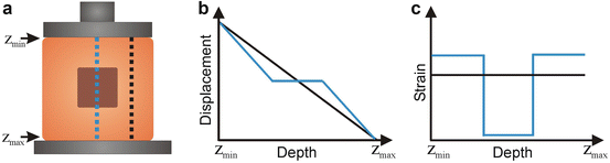
The basic principle of compression OCE is illustrated in Fig. 32.7. A soft material containing a stiff inclusion, resting on a rigid, immovable surface, is subjected to a step load by an external compression plate. The displacement versus depth introduced at the positions indicated by the black and blue lines in Fig. 32.7a is shown in Fig. 32.7b. The displacement in the homogeneous region of the sample (black line) decreases linearly to zero at z max, i.e., the sample undergoes uniform compression. The displacement through the center of the sample (blue curve) shows a local deviation in the displacement in the region corresponding to the stiff inclusion. Assuming the inclusion has a Young’s modulus much larger than the background material, it can be considered to displace as a bulk, i.e., the displacement at each position in the inclusion is equal.