Fig. 1.1
Optical coherence tomography (OCT) generates cross-sectional or three-dimensional images by measuring the magnitude and echo time delay of light. Measurements of backreflection or backscattering versus depth known as axial scans (A-scans). Cross-sectional images are generated by scanning the OCT beam in a transverse direction to acquire a series of axial scans. This generates a two-dimensional data set (B-scan) which can be displayed as a gray scale or false color image. Three-dimensional volumetric data sets (3D-OCT) can be acquired by raster scanning to generate a series of two-dimensional data sets (B-scans)
OCT is a powerful medical imaging technology because it performs “optical biopsy,” the real time, in situ visualization of tissue microstructure and pathology, without the need to remove and process specimens [2, 3]. Although histopathology is the gold standard for assessing pathology, it requires excision, fixation, embedding, microtoming, and staining of tissue specimens. OCT has applications in several general clinical situations: (1) Where standard excisional biopsy is hazardous or impossible. Applications include tissues such as the eye, arteries, or nervous tissues. (2) Where standard excisional biopsy has sampling error. Excisional biopsy and histopathology is used for diagnosis of many diseases including cancer; however, if the biopsy misses the lesion, this causes a false negative. OCT can guide excisional biopsy to reduce the number of biopsies required and to improve sensitivity by reducing sampling errors. If sufficient sensitivities and specificities can be achieved, OCT may be used to diagnose pathology in real time. Since imaging is performed in situ, OCT has the advantage that much larger regions of tissue can be assessed than by excisional biopsy. (3) For guidance of interventional procedures. In ophthalmology, OCT can visualize changes in retinal structure and markers of disease such as neovascularization or edema to assess pharmaceutical treatment response. In cardiology and intravascular imaging, the ability to see cross-sectional and three-dimensional structure enables the guidance of procedures such as stent placement. The ability to see beneath the tissue surface enables guidance of ablative therapies such as laser or radio-frequency ablation, as well as surgical and microsurgical procedures. (4) For performing functional measurement and imaging. Doppler OCT enables quantitative measurement of blood flow. Complementary methods such as OCT angiography enable three-dimensional imaging of vascular structure using motion contrast from moving blood cells. Polarization-sensitive OCT enables measurement of birefringence, a marker for cellular and subcellular organization. Spectroscopic, displacement, vibrometry, and many other measurements are possible. Although the imaging depth of OCT is limited by attenuation from light scattering, OCT can be integrated with many medical devices such as catheters, endoscopes, laparoscopes, or needles, to access luminal organ systems such as the GI tract and airway as well as solid organs and masses.
OCT has become a standard of care in clinical ophthalmology and promises to have a powerful impact on many medical applications ranging from intravascular imaging to the assessment of neoplasia and guidance of minimally invasive surgical procedures. This chapter reviews the background and development of OCT.
1.2 OCT and Ultrasound
OCT has features which are common to both ultrasound and microscopy. In order to understand OCT imaging, it is helpful to compare it with these related medical imaging techniques. Figure 1.2 shows the resolution and imaging depth for several imaging modalities. The resolution of clinical ultrasound imaging is typically 0.1–1 mm and depends on the frequency of the sound wave (3–40 MHz) used for imaging [4–6]. Sound waves at standard ultrasound frequencies are transmitted with minimal absorption in biological tissue and it is possible to image structures deep in the body. High frequency ultrasound has been used for research and clinical applications such as intravascular imaging. Resolutions of 15–20 μm and finer have been achieved with frequencies of ∼100 MHz. However, these high frequencies are strongly attenuated in biological tissues and imaging depths are limited to only a few millimeters.
Fig. 1.2
Comparison of ultrasound, OCT, and confocal microscopy resolution and imaging depth. Standard clinical ultrasound achieves deep imaging depths, but has limited resolution. Higher sound frequencies yield finer resolution, but ultrasonic attenuation increases, reducing image penetration. OCT axial image resolution ranges from 1 to 15 μm, determined by the coherence length of the light source. In most biological tissues attenuation from optical scattering limits OCT imaging depth to 2–3 mm. Confocal microscopy has submicron resolution, but imaging depth is only a few hundred microns in most tissues
Microscopy and confocal microscopy are examples of imaging techniques which have extremely high transverse image resolutions of 1 μm or finer. Imaging is typically performed in an en face plane and resolutions are determined by optical diffraction. The imaging depth in biological tissue is limited because image signal and contrast are significantly degraded by unwanted scattered light. In most biological tissues, imaging can be performed to depths of only a few hundred microns.
OCT fills a gap between ultrasound and microscopy. The axial image resolution in OCT is determined by the bandwidth of the light source. OCT technologies have axial resolutions ranging from 1 to 10 μm, approximately 10–100 times finer than standard ultrasound imaging. The high resolution of OCT imaging enables the visualization of tissue architectural morphology. OCT has become a clinical standard in ophthalmology, because the transparency of the eye provides easy optical access to the retina and noncontact high-resolution imaging is possible [7]. The major limitation of OCT is that light is highly scattered by most tissues and attenuation from scattering limits the imaging depths to ∼2 mm in most tissues. However, because OCT uses fiber optics, it can be integrated with a wide range of medical instruments such as catheters, endoscopes, laparoscopes, or needles which enable imaging in luminal organ systems or even solid tissues inside the body.
OCT imaging is analogous to ultrasound imaging except that it uses light instead of sound. There are several different detection methods for performing OCT, but essentially imaging is performed by measuring the magnitude and echo time delay of backreflected or backscattered light from internal microstructures in materials or tissues. OCT images are two-dimensional or three-dimensional data sets which represent optical backreflection or backscattering in a cross-sectional plane or 3D volume. Ultrasound and OCT are analogous in that when a beam of sound or light is incident into tissue, it is backreflected or backscattered differently from structures which have varying acoustic or optical properties, as well as from boundaries between structures. The dimensions of these internal structures can be determined by measuring the “echo” time it takes for sound or light to travel different axial distances.
In ultrasound, the axial measurement of distance or depth is called A-mode scanning, while cross-sectional imaging is called B-mode scanning. Volumetric or 3D imaging can be performed by acquiring multiple B-mode images. The principal difference between ultrasound and optical imaging is that the speed of light is extremely high. The speed of sound is ∼1,500 m/s, while the speed of light is approximately 3 × 10⁸ m/s. In order to measure distances with a 100 μm resolution, a typical resolution for ultrasound imaging, a time resolution of ∼100 ns is required. This resolution is well within the limits of electronic detection. Ultrasound technology has advanced significantly in recent years with the availability of high-performance, low-cost analog to digital converters and digital signal processing technology. Unlike sound, the detection of light echoes requires much higher time resolution. Light travels from the moon to the earth in only ∼2 s. The measurement of distances with a 10 μm resolution, a typical resolution for OCT imaging, requires a time resolution of ∼30 fs (30 × 10−15 s). A femtosecond is extremely fast; the ratio of 1 fs–1 s is equal to the ratio of 1 s to the time since the age of dinosaurs. Direct electronic detection is impossible with this time resolution and measurement methods such as high-speed optical gating, optical correlation, or interferometry must be used.
1.3 Measuring Optical Echoes
1.3.1 Photographing Light in Flight
Using optical echoes to see through biological tissue was proposed by Michel Duguay, more than 30 years ago, in 1971 [8, 9]. These pioneering studies demonstrated an ultrafast optical shutter based on the laser-induced Kerr effect which could “photograph light in flight.” Figure 1.3 shows a schematic of the ultrahigh-speed Kerr shutter and an ultrashort light pulse propagating though a scattering solution of diluted milk [9]. The Kerr shutter operates by using an intense laser pulse to induce birefringence (the Kerr effect) in an optical medium placed between two crossed polarizers. If the induced birefringence is electronically mediated, it has an extremely rapid response time and the Kerr shutter can achieve picosecond or femtosecond time resolution.
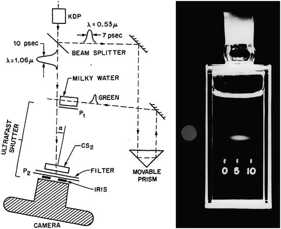
Fig. 1.3
Photographing light in flight. (left) A high-speed optical shutter is created using a CS2 cell placed between crossed polarizers. An intense laser pulse induces transient birefringence (the Kerr effect) and opens the shutter (right). Photograph of an ultrashort laser pulse propagating through a cell of milk and water. The shutter speed was 10 ps. These early studies suggested that high-speed optical gating could be used to see inside biological tissues by rejecting unwanted scattered light (Duguay and Mattick [9])
Optical scattering limits the ability to image biological tissues, and Duguay proposed that an ultrahigh-speed shutter could remove unwanted scattered light and detect light echoes from inside tissue [9]. Ultrahigh-speed optical shutters might be used to “see through” tissues and noninvasively image internal pathology. The major limitation of the high-speed optical Kerr shutter is that it requires high intensity, short laser pulses to induce the Kerr effect and operate the shutter.
1.3.2 Femtosecond Time Domain Measurement
An alternate method for detected optical echoes is to use nonlinear optical processes such as harmonic generation, sum frequency generation, or parametric conversion [10–12]. Short pulses illuminate the tissue and the backscattered light is nonlinearly mixed with a reference pulse in a nonlinear optical material. The nonlinear process can measure the intensity and time delay of the optical signal with a time resolution determined by the pulse duration. Figure 1.4 shows a schematic of how transient light echoes are detected using nonlinear second harmonic generation cross correlation. The reference pulse is generated by the same laser source and is delayed by a variable time delay ΔT using a mechanical optical delay line. The nonlinear mixing process creates an ultrahigh-speed optical gate. If IS(t) is the signal that is being detected and Ir(t) is the reference pulse used as the gate, the response function S(ΔT) is
Fig. 1.4
Early demonstration of femtosecond optical ranging in biological systems. (left) Femtosecond echoes of backscattered light (signal) are detected using nonlinear second harmonic generation, mixing the signal with a delayed reference pulse. (right) Measurement of corneal thickness in an in vivo rabbit eye using femtosecond pulses, showing an axial scan of backscattering versus depth. An axial resolution of 15 μm (in air) was achieved using a femtosecond dye laser generating 65 fs pulses at 625 nm wavelength. The detection sensitivity was −70 dB or 10−7 (From Fujimoto et al. [12])
Figure 1.4 shows a measurement of corneal thickness in a rabbit eye in vivo. Very low scattering from the corneal stroma can be detected. The measurement had a 15 μm axial resolution and was performed using 65 femtosecond duration pulses from a femtosecond dye laser at 625 nm wavelength. Sensitivities of −70 dB or 10−7 of the incident intensity were achieved. However, these sensitivities were still not high enough to image most biological tissues. Current OCT systems achieve sensitivities 1,000× higher, approaching −100 dB or 10−10 of the incident intensity.
1.3.3 Low-Coherence Interferometry
Interferometry is a powerful technique for measuring the magnitude and echo time delay of backscattered light with very high sensitivity. OCT is based on a classic optical measurement technique known as low-coherence interferometry, or white light interferometry, first described by Sir Isaac Newton. Low-coherence interferometry was used in photonics to measure optical echoes and backscattering in optical fibers and waveguide devices in the 1980s [13–15]. The first biological application of low-coherence interferometry for the measurement of axial eye length was reported by Fercher et al. in 1988 [16]. Different versions of low-coherence interferometry were developed for noninvasive measurement in biological tissues [17–20].
Interferometry techniques perform correlation measurements by interfering light that is backscattered from the tissue with light that has traveled through a reference path with a known time delay. Also, interferometry measures the electric field of the light wave rather than its intensity. Figure 1.5 shows a schematic diagram of a classic Michelson interferometer. The incident light source is divided into a reference beam Er(t) and a measurement or signal beam Es(t) which travel different distances in the two interferometer arms. The electric field of the interferometer output is the sum of the signal and reference fields, Er(t) + Es(t), and a detector measures the output intensity, which is proportional to the square of the total field:
Fig. 1.5
Low-coherence interferometry. (left) Backreflected or backscattered light is interfered with light from a scanning reference path delay. Using low-coherence length light, interference only occurs when the path lengths are matched to within the coherence length. The interferometer output is detected as the reference path delay is scanned (time domain detection). The echo magnitude versus delay or axial scan is obtained by demodulating the interference signal. (right) Measurement of the anterior chamber in an ex vivo bovine eye. A 10 μm axial resolution was achieved using a low-coherence diode light source at ∼800 nm. Interferometry enables high sensitivity detection of optical echoes and is the basis for optical coherence tomography (From Huang et al. [21])
ΔL is the path length difference between the signal and reference arms of the interferometer. If the reference path length is scanned, interference fringes will be generated as a function of time. This process can also be understood by noting that the scanning reference arm produces a Doppler shift of the reference field. If a coherent (narrow linewidth) light source is used, interference will be observed over a wide range of path length differences. However, in order to detect optical echoes, a low-coherence (broad bandwidth) light source is required. Low-coherence light can be characterized as having statistical phase discontinuities over a distance known as the coherence length, which is inversely proportional to the frequency bandwidth of the light. When low-coherence light is used, interference is only observed when the measurement and reference path lengths are matched to within the coherence length. The interferometer essentially measures the field autocorrelation of the light wave. The magnitude and echo time delay of light echoes can be measured by scanning the reference arm and demodulating, detecting the envelope of the interference signal. The coherence length of the light source determines the axial image resolution. Shorter coherence lengths from broadband light sources provide finer resolution.
Figure 1.5 shows an early ex vivo measurement of the anterior chamber of the bovine eye with a 10 μm axial resolution using an 800 nm wavelength, low-coherence diode light source with a bandwidth of 29 nm [21]. Sensitivities of −100 dB or 10−10 of the incident intensity were achieved. Scanning the beam in the transverse direction yielded information on different structures, such as the lens and iris. The axial measurements of backscatter versus depth using low-coherence interferometry provided the foundation for optical coherence tomography. Low-coherence interferometry has the advantage that can be performed with continuous wave light sources, without requiring short pulse lasers. Since interferometry measures the field rather than the intensity, it is equivalent to heterodyne detection in optical communication. Weak signals Es(t) are multiplied by a strong reference field Er(t) to produce heterodyne gain and very high, shot noise-limited sensitivities can be achieved. In addition, since the intensity is the square of the field, very high dynamic ranges are possible.
1.4 The Development of OCT
1.4.1 Early OCT Technology and Systems
Optical coherence tomography imaging was demonstrated in 1991 by Huang et al. [1]. Figures 1.6 and 1.7 show the first OCT images of the retina and human coronary artery ex vivo with corresponding histology [1]. These examples demonstrate OCT imaging in transparent as well as optically scattering tissues. Imaging was performed with 15 μm axial resolution in tissue at 830 nm wavelength. The image is displayed using a log false color scale with a signal level ranging between ∼ −60 and −90 dB of the incident intensity. The OCT image of the retina in Fig. 1.6 shows the contour of the optic nerve head as well as retinal vasculature near the nerve head. The retinal nerve fiber layer can also be visualized emanating from the optic nerve head. This image was ex vivo and postmortem retinal detachment is evident. The OCT image of the coronary artery in Fig. 1.7 shows fibrocalcific plaque on the right of the specimen and fibroatheromatous plaque on the left. The plaque scatters light and therefore attenuates the OCT beam, limiting the image penetration depth. Ophthalmic and intravascular imaging have emerged as two of the major applications of OCT which are now in clinical practice.
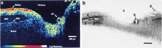
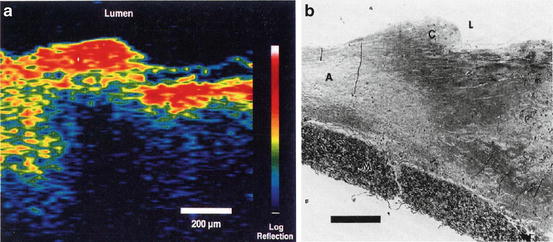
Fig. 1.6
OCT image of the human retina ex vivo and corresponding histology. Imaging was performed with 15 μm axial resolution in tissue at 830 nm wavelength. The OCT image is displayed using a log false color scale spanning –60 to –90 dB of the incident light intensity. The image shows the optic nerve head contour and vasculature. The retinal nerve fiber layer can be visualized and there is postmortem retinal detachment with subretinal fluid accumulation (From Huang et al. [1])
Fig. 1.7
OCT image of human artery ex vivo and corresponding histology. The OCT image shows fibrocalcific plaque (right three-quarters of specimen) and fibroatheromatous plaque (left). The fatty-calcified plaque scatters light and attenuates the OCT beam, limiting the image penetration depth (From Huang et al. [1])
Optical coherence tomography has the advantage that it can be implemented using fiber-optic components and integrated with a wide range of medical instruments. OCT systems can be divided into an imaging engine (consisting of an interferometer, light source, and detector) and imaging devices or probes. Early OCT imaging engines employed time domain detection with an interferometer using a low-coherence light source and scanning reference arm delay. Figure 1.8 shows an example of an OCT system using a fiber-optic Michelson-type interferometer with time domain detection. A low-coherence light source is coupled into the interferometer. One arm of the interferometer emits a beam which is directed and scanned on the sample being imaged, while the other arm is a reference with a scanning delay. The interferometer shown in Fig. 1.8 uses a circulator to collect the interference signal which returns to the light source to improve efficiency. This interference signal is out of phase with the other interferometer output. When these two signals are subtracted, the desired interference signal adds and excess noise from the light source is cancelled. This configuration is known as dual balanced detection and is used in coherent optical communications systems [22]. There are many different embodiments of the interferometer and imaging engine which have different power delivery and detection efficiency advantages [23]. Chapter 11, “Optical Design for OCT,” discusses aspects of OCT system design in more detail.
Fig. 1.8
OCT imaging system based on a fiber-optic Michelson interferometer. OCT has the advantage that it uses photonics and fiber optics technology. This schematic shows a Michelson interferometer with a circulator for dual balanced detection. Dual balanced detection adds the signal from the interference of the sample and reference arms and subtracts excess noise from the light source. The sample/probe arm may be interfaced to a variety of imaging devices. OCT interferometers can be built in many different configurations depending on design requirements
Because the eye is optically accessible and optical imaging methods are widely used in ophthalmology, many of the earliest OCT studies were in the eye. The first in vivo retinal images were obtained independently in 1993 by Fercher et al. [24] and Swanson et al. [25]. Figure 1.9 shows an early in vivo OCT image of the normal human retina from Hee et al. in 1995 [26]. Imaging was performed at 800 nm wavelength with ∼10 μm axial resolution in tissue. The nerve fiber layer as well as other architectural features can be visualized with higher resolution than was previously possible. Several thousand patients were imaged at the New England Eye Center in the mid-1990s. These early clinical studies investigated OCT for the diagnosis and monitoring of a variety of macular diseases [27], including macular edema [28, 29], macular holes [30], central serous chorioretinopathy [31], and age-related macular degeneration and choroidal neovascularization [32]. The retinal nerve fiber layer thickness, an indicator of glaucoma, can be quantified in normal and glaucomatous eyes and correlated with conventional measurements of the optic nerve structure and function [33,34]. Many of the measurement protocols that were developed in these early studies were adopted in current OCT ophthalmic instruments [7].
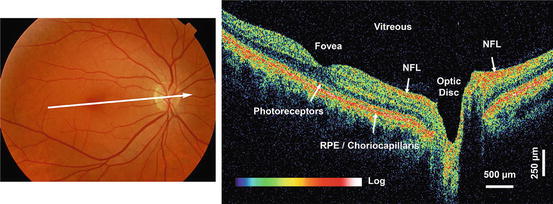
Fig. 1.9
Early in vivo OCT image of the normal retina in a human subject. Imaging was 10 μm axial resolution at 800 nm wavelength. The retinal pigment epithelium, choroid, and retinal nerve fiber layers are visible as highly backscattering layers. OCT can noninvasively visualize and quantitatively measure retinal pathology and is now a standard of care in clinical ophthalmology (From Hee et al. [26])
The high detection sensitivity of OCT enables imaging structures such as the retina which have very low optical scattering. Typical retinal images have signal levels of −50 to −90 dB of the incident intensity. For retinal imaging, safety standards govern the maximum permissible light exposure and set limits for OCT imaging speeds [25, 26]. However, the majority of OCT applications require imaging in tissues which are not transparent, but instead are highly scattering. In this case, detection sensitivity is also important because light is highly attenuated by scattering and the sensitivity determines the imaging depth.
OCT imaging in tissues other than the eye became feasible with the recognition that using longer optical wavelengths can reduce scattering and increase image penetration depths [3, 35, 36]. Figure 1.10 shows an early example from Brezinski et al. 1996 showing OCT imaging in a human epiglottis ex vivo, comparing imaging at 850 nm and 1,300 nm wavelengths [3]. The dominant absorbers in most tissues are melanin and hemoglobin, which have absorption at visible and near-infrared wavelengths [37]. Water absorption becomes dominant for longer wavelengths, approaching 1,900–2,000 nm. In most tissues, scattering at near-infrared wavelengths is one to two orders of magnitude higher than absorption, and scattering decreases for longer wavelengths. Therefore, imaging at 1,300 nm improved image penetration and has become a standard wavelength for most non-ophthalmic OCT applications.
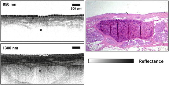
Fig. 1.10
OCT imaging penetration depth. OCT in scattering tissues was made possible using longer wavelengths which are less attenuated by scattering. OCT images of human epiglottis ex vivo performed with 850 nm and 1,300 nm wavelengths. Superficial glandular structures (g) can be seen in images with 850 nm and 1,300 nm wavelengths, but the underlying cartilage (c) is better visualized with longer 1,300 nm wavelength. With a detection sensitivity of ∼90–100 dB, image penetration depths of up to 2–3 mm are possible in most scattering tissues (From Brezinski et al. [3])
Early studies investigated the mechanisms of OCT image contrast as they are related to tissue optical properties [35, 38]. Chapter 3, “Modeling Light–Tissue Interaction in Optical Coherence Tomography Systems” considers these mechanisms in detail. In OCT images, tissue structures are visible because they have different optical scattering properties. OCT images show true tissue dimensions (correcting for index of refraction and beam refraction effects); however, if OCT is displayed using a false color image, the colors represent different optical properties and not necessarily different tissue morphologies. In histology, histological sections are stained in order to produce selective contrast between different tissue structures. There are multiple stains available for histology which are highly specific. OCT relies on intrinsic differences in optical properties of different tissues in order to produce image contrast. On one hand this is a limitation because tissue structures, for example, nuclei of cells, may not have contrast in OCT imaging. However, histology is a time-consuming process which requires tissue excision, processing, embedding, sectioning, and staining, while OCT imaging can be performed on tissue in situ and in real time, without the need for excision and processing.
Several early OCT imaging studies were performed using ex vivo surgical specimens [3, 39–50]. These studies helped to define which structural features were visible using OCT and to establish a baseline for comparison to histology. Figure 1.11 shows an example of one of the first OCT images of arterial plaque ex vivo and corresponding histology from Brezinski et al. 1996 [3]. The OCT image has an axial resolution of ∼15 μm in tissue and imaging was performed at 1,300 nm wavelength. The figure shows an unstable plaque characterized by a thin intimal cap layer, adjacent to a heavily calcified plaque with low lipid content. The demonstration that OCT could resolve unstable plaque in ex vivo specimens was an important milestone which helped lead to the later clinical development of intravascular OCT imaging.
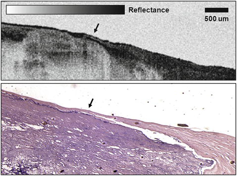
Fig. 1.11
Early OCT image of atherosclerotic plaque ex vivo and corresponding histology. The plaque is highly calcified with relatively low lipid content and a thin intimal cap. This result demonstrated that OCT can resolve morphological features associated with unstable plaques (From Brezinski et al. [3])
Another active area of OCT research is the detection of neoplastic changes. Early studies were performed ex vivo to correlate OCT images with histology for gastrointestinal [40, 41, 44, 50], biliary [45], female reproductive [47, 49], pulmonary [46], and urinary [42, 48] pathologies. Figure 1.12 shows an example from an early OCT imaging study of gastrointestinal neoplasia. The figure shows OCT images and corresponding histology of normal colon and adenocarcinoma ex vivo. Imaging was performed with an axial resolution of ∼15 μm in tissue at 1,300 nm wavelength. The OCT image of normal colon shows normal glandular organization associated with columnar epithelial structure. The mucosa and muscularis mucosa can be differentiated by the different backscattering characteristics within each layer. Architectural morphology, such as crypts or glands within the mucosa, can be visualized. The OCT image of adenocarcinoma shows disruption of architectural morphology or glandular organization. However, assessing cancer pathology is an extremely challenging application. OCT has significant limitations in both tissue contrast and resolution compared with the gold standard of excisional biopsy and histopathology. These challenges have been a factor in the slower development of OCT for cancer applications.
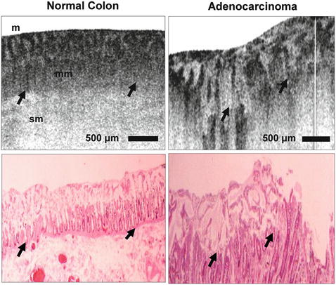
Fig. 1.12
OCT imaging of neoplastic changes. Early ex vivo OCT image of normal colon (left) and adenocarcinoma (right) with corresponding histology. The mucosal (m), muscularis mucosa (mm), and submucosal (sm) layers of the normal colon are visible. Dilated and disorganized crypts (c) are visible in the specimen with adenocarcinoma. OCT can visualize changes in architectural morphology (Pitris et al. [50])
1.4.2 Ophthalmic OCT Imaging
The earliest clinical studies with OCT were performed in ophthalmology, and to date OCT has had the largest clinical impact in this specialty. OCT is a powerful technique in ophthalmology because it can identify markers of early disease at treatable time points before visual symptoms and irreversible vision loss occurs. Furthermore, repeated imaging can be performed to track disease progression or monitor the response to therapy. The development of a prototype clinical instrument was a key step to enabling early studies in ophthalmology. Figure 1.13 shows a photograph of an early prototype instrument for OCT retinal imaging that was designed and built by Eric Swanson at MIT Lincoln Laboratories in the mid-1990s. The instrument was based on a slit lamp biomicroscope and provided a simultaneous view of the retinal fundus for aiming and registering the OCT imaging beam. This instrument was used in the New England Eye Center to perform the first clinical studies of OCT in ophthalmology [25–27, 51]. Several thousand patients were imaged in cross-sectional as well as longitudinal studies during the mid-1990s.
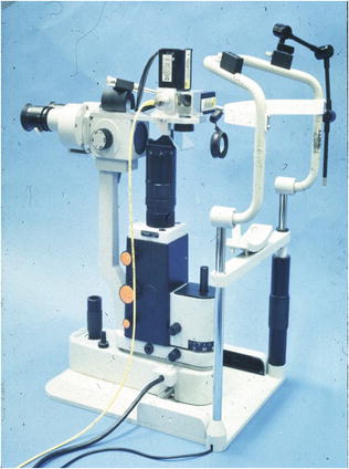
Fig. 1.13
Photograph of an early retinal imaging prototype instrument. The OCT system is interfaced with a slit lamp biomicroscope. The OCT beam is scanned using a pair of galvanometer-actuated mirrors. This system was used at the New England Eye Center and imaged several thousand patients during the mid-1990s (Courtesy of Eric Swanson)
Figure 1.14 shows a schematic diagram of the optical design for retinal imaging. Similar design principles were used for OCT using low numerical aperture microscopes imaging developmental biology specimens in vivo as well as for surgical imaging applications [39, 52, 53]. An objective lens relays an image of the retina onto an intermediate image plane where it can be viewed by the operator or a video camera. The OCT beam is coupled into the instrument using a beam splitter and focused onto the intermediate image plane using a relay lens and then imaged onto the retina by the objective lens and the subject’s eye. The transverse spot size of the OCT beam on the retina is typically ∼20 μm and is limited by ocular aberrations. The transverse position of the OCT beam is scanned by two perpendicular x-y galvanometer scanning mirrors. The optical system is designed so that the beam pivots about the pupil of the eye when it is scanned. This prevents the OCT beam from being vignetted by the pupil and enables a wide field of view on the retina. OCT imaging can be performed at different locations on the retina by controlling the scanning of the OCT beam. When the OCT beam is scanned, it is visible on the retina that is visible to the operator, enabling aiming. The OCT beam is also visible to the patient as a small spot or scanned line, whose position in the patient’s visual field corresponds to the points on the retina that are being scanned. Since the scanning trajectory of the OCT beam on the retina can be controlled, different scan patterns can be designed and adopted as part of the diagnostic protocol for specific retinal diseases.
Fig. 1.14
Schematic of OCT instrument design for retinal imaging. An objective lens relay images the retina to a plane in the OCT instrument. Operator viewing of the fundus is performed by imaging with a video camera. Computer-controlled galvanometer scanning mirrors positions and scan the OCT beam. A relay lens focuses the OCT beam onto the image plane, and the objective lens directs the OCT beam through the pupil onto the retina. The OCT beam is focused on the retina by adjusting the objective lens. The OCT beam pivots about the pupil of the eye in order to minimize vignetting
OCT is important for the diagnosis and monitoring of diseases such as glaucoma, age-related macular degeneration, and diabetic retinopathy because it provides quantitative information on retinal pathology which is a measure of disease progression or response to therapy [29, 33, 54]. Images can be analyzed quantitatively and processed using intelligent algorithms to extract features such as retinal or retinal nerve fiber layer thickness. Mapping and display techniques have been developed to display OCT data in alternate forms, such as thickness maps, in order to aid interpretation. Figure 1.15 shows an early example of an OCT topographic map of retinal thickness [29]. The thickness map was constructed by performing six standard OCT scans at varying angular orientations through the fovea. The OCT images are segmented to detect the retinal thickness which is then linearly interpolated over the macular region and represented as a false color topographic map. For quantitative interpretation, the macula is divided into different regions and averaged values of retinal thickness are displayed. The ability to reduce image information to numerical information is important because it enables the development of normative databases and the use of statistical criteria for disease diagnosis.
Fig. 1.15
OCT topographic map of retinal thickness. (Top) OCT image of the macula which has been segmented in order to measure retinal thickness. The anterior and posterior retinal surfaces are automatically identified. (Middle) Quantitative measurement of retinal thickness based on the segmented OCT image. (Bottom) Topographic map of macular retinal thickness. The topographic map is constructed by segmenting multiple OCT scans which are radially oriented in the macula, measuring the retinal thickness, and interpolating the retinal thickness in the regions between the scans. Retinal thickness is represented by a color table and has the advantage that it can be directly compared with the retinal fundus image
OCT technology was transferred to industry by our group at MIT and introduced commercially for ophthalmic diagnostics in 1996 (Carl Zeiss Meditec). Early instruments had an axial resolution of 10 um and an imaging speed of 100 A-scans/s. A third generation ophthalmic instrument, the Stratus OCT, was introduced in 2002 which had similar resolution, but faster speed of 400 A-scans/s. The increased speed enabled an increase in image pixel density. The large amount of published clinical data from previous generation instruments, coupled with technological improvements and reimbursement, helped the clinical adoption of OCT. By the mid-2000s, OCT became a standard of care in ophthalmology and is considered essential for the diagnosis and monitoring of many retinal diseases [7]. With increases in imaging speed provided by spectral/Fourier domain detection, many companies entered the ophthalmic marketplace in the mid-2000s.
1.4.3 Catheter and Endoscopic OCT Imaging Technology
Flexible imaging probes such as catheters and endoscopes were key to enabling internal body OCT imaging [55, 56]. Figure 1.16 shows one of the first OCT catheter/endoscopes devices. This device was a prototype for modern OCT intravascular imaging catheters and endoscopic probes. The catheter/endoscope has a single-mode optical fiber in a hollow rotating torque cable, coupled to a distal lens and microprism that reflects the OCT beam radially. The torque cable and distal optics are contained in a transparent housing. The OCT beam is scanned by rotating the torque cable to generate a transverse image in luminal structures or hollow organs. Imaging may also be performed in a longitudinal plane by push-pull movement or a spiral rotation and pullback of the torque cable assembly [57]. The early catheter/endoscope shown in Fig. 1.16 had a diameter of 2.9 French or 1 mm, similar to a standard IVUS catheter. The development of catheter imaging devices is challenging because of the simultaneous mechanical, optical, and biocompatibility requirements. Early commercial devices (such as the LightLab Imaging ImageWireTM and HeliosTM occlusion balloon catheters) used micro-optic fabrication methods to create lenses and beam-directing elements which have diameters of optical fibers (80–250 μm), significantly smaller than can be achieved with IVUS catheters.
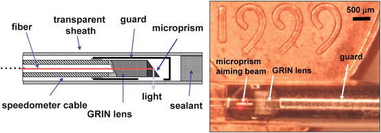
Fig. 1.16
Catheter/endoscopic OCT imaging. Schematic and photograph of an early OCT catheter/endoscope for intraluminal imaging. A single-mode fiber is contained in a rotating flexible speedometer cable which is enclosed in a protective plastic sheath. The distal end has a lens and prism/mirror which focuses the beam at 90° from the catheter axis. The diameter of the catheter is 2.9 French or ∼1 mm. The catheter is shown on a United States coin for scale. OCT can be integrated with a wide range of diagnostic and interventional devices
1.4.4 Intravascular OCT Imaging
Intravascular imaging is the second most developed clinical OCT application. Figure 1.17 shows the first catheter-based image of a human coronary artery ex vivo using an early prototype 2.9 F OCT catheter, from Tearney et al. in 1996 [58]. The figure shows a comparison of OCT with 30 MHz intravascular ultrasound (IVUS). The OCT image shows excellent differentiation of the intima, media, and adventitia and suggested the utility of intravascular OCT. In vivo intravascular OCT imaging was challenging because of the need to develop suitable catheter imaging devices which could be used in animals and human subjects. In addition, since blood is highly optically scattering, it was necessary to develop saline/contrast flushing or balloon occlusion protocols to remove blood or to significantly dilute the hematocrit in the imaging field. Intravascular OCT animal imaging studies were performed in a rabbit model by Fujimoto et al. in 1999 [59]. Imaging was performed using a 2.9 F optical catheter using a time domain OCT system with a broadband femtosecond laser at 1,280 nm wavelength to achieve 10 um axial resolution. Imaging speeds were 4 frames/s with a 512 axial pixel images. Because blood is highly optically scattering at normal hematocrit, saline flushing was required to dilute the hematocrit during imaging. Intravascular animal imaging studies were performed in a porcine model using saline flushing by Tearney et al. in 2000 [60]. This study reported OCT imaging of normal coronary arteries, intimal dissections, and stents with 10 μm resolution.
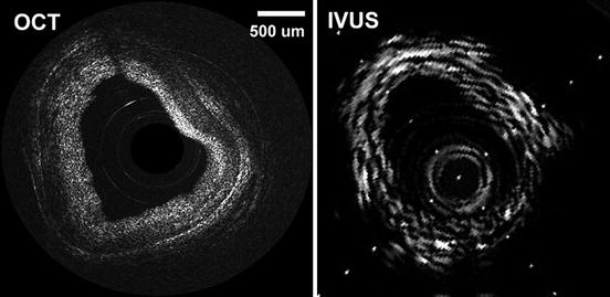
Fig. 1.17
Early OCT image of a human artery ex vivo and comparison with intravascular ultrasound (IVUS). The OCT image has 15 μm axial resolution and enables the differentiation of the intima, media, and adventitia. Intimal hyperplasia is evident. IVUS has deeper image penetration, but lower resolution (From Tearney et al. [58])
OCT imaging in human patients was first reported by Jang et al. in 2001 [61]. This pioneering study used a 3.2 F OCT imaging catheter and demonstrated imaging of tissue prolapse in a stent, comparing OCT with IVUS. The study was a significant landmark because it addressed multiple technological, clinical, and administrative challenges. Independent clinical demonstrations by Grube et al. at the Siegburg Heart Center were reported in 2002 using a prototype instrument developed by LightLab Imaging [62]. Other early studies compared OCT with IVUS for visualization of stent placement and apposition [63, 64]. Figure 1.18 shows an early example of intravascular OCT imaging of a partially restenosed stent with a corresponding l-mode pullback image (courtesy of Osaka City University Hospital and LightLab Imaging). This image was acquired using an occlusion balloon catheter and shows neointimal growth over a stent. Modern intravascular OCT instruments use flushing with contrast agents to dilute hematocrit combined with high-speed imaging.
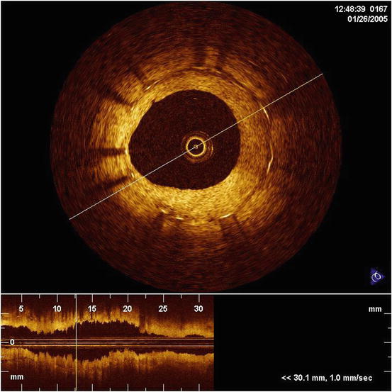
Fig. 1.18
Intravascular OCT. Early OCT image and pullback of a stent with neointimal growth in a human artery in vivo. Saline flushing was used to remove blood from the imaging field. Imaging was performed with the LightLab M2 and an occlusion balloon catheter. Modern intravascular OCT instruments use contrast flushing without occlusion (Courtesy of LightLab Imaging)
Intravascular OCT imaging is currently an active area of both research and commercialization. The commercial development of intravascular OCT was performed by an MIT startup in 1998. The first commercial intravascular OCT instrument generated images with 200 A-scans at 15 frames/s and was introduced in Europe in 2004. A higher performance system with 240 A-scan per frame at 20 frames/s was introduced in 2007. A system based on swept source/Fourier domain detection achieved 500 A-scans per frame at 100 frames per second, and FDA approval was obtained in 2010. Chapters 69, “Imaging Coronary Atherosclerosis and Vulnerable Plaques with Optical Coherence Tomography” and 70, “Cardiovascular Optical Coherence Tomography” describe intravascular OCT in more detail. Chapter 71, “Intravascular OCT” discusses the process of commercialization of OCT from the perspective of intravascular imaging.
1.4.5 Endoscopic OCT and Cancer Detection
The first demonstrations of in vivo endoscopic OCT imaging were performed in 1997 [56, 65]. Figure 1.19 shows an example of OCT imaging of the rabbit esophagus in vivo and corresponding histology, from Tearney et al. [56]. This image demonstrates visualization of the esophageal layers including the mucosa (m), the submucosa (sm), the inner muscularis (im), outer muscularis (om), and serosa (s). The first clinical studies of endoscopic OCT imaging in human subjects were reported by Sergeev et al. in 1997 [65] and Feldchtein et al. in 1998 [66]. OCT imaging was performed with a flexible forward scanning probe in the working channel of a standard endoscope, bronchoscope, or trocar. The imaging device was a 1.5–2 mm diameter probe which used a miniature magnetic scanner to image in the forward direction. These early studies demonstrated the feasibility of performing clinical OCT imaging of organ systems such as the esophagus, larynx, stomach, urinary bladder, and uterine cervix.
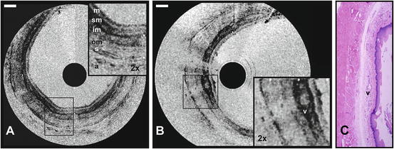
Fig. 1.19
Endoscopic OCT image of the rabbit esophagus in vivo demonstrating internal body imaging. (a) Esophageal layers including the mucosa (m), submucosa (sm), inner muscular layer (im), outer muscular layer (om), serosa (s), and adipose and vascular supporting tissues (a) can be visualized. (b) A blood vessel (v) can be seen within the submucosa. (c) Corresponding histology. Scale 500 um (Tearney et al. [56])
Gastrointestinal (GI) endoscopy received considerable attention due to the prevalence of esophageal, stomach, and colon cancers. In contrast to conventional endoscopy that visualizes surface features, OCT can image subsurface tissue morphology. Early studies of endoscopic OCT imaging suggested the ability of OCT to differentiate GI pathologies such as the Barrett’s esophagus, adenomatous polyps, and adenocarcinoma [57, 65, 67–73]. However, the development of OCT imaging for cancer detection remains extremely challenging. Conventional histopathology is an extremely powerful diagnostic technique because it enables the use of selective stains to enhance contrast between different cellular or tissue structures. Histology also provides extremely fine image resolutions, enabling the visualization of not only larger scale tissue architectural morphology but also subcellular structure. OCT imaging relies on intrinsic contrast produced by variations in scattering properties of different tissue structures. On the positive side, OCT enables real time imaging of tissue pathology in situ, without the need for excision and processing as in conventional biopsy and histopathology. When used to guide biopsy, it is not necessary for OCT to perform at the level required for diagnosis, but it must have sufficient sensitivity to detect pathology and improve the sensitivity of excisional biopsy by reducing sampling errors.
The development of OCT for cancer detection will require detailed clinical studies which investigate its ability to identify relevant pathologies. These types of studies are challenging because the sensitivity and specificity of OCT imaging must be evaluated relative to biopsy and histopathology which is the gold standard for diagnosis. Since pathology varies depending upon location, precise registration of OCT imaging and excisional biopsy is required. This is an especially challenging problem in endoscopic applications. Sufficient numbers of patients having a given pathology must be investigated in order to ensure that the sample size is large enough to generate statistically significant results. Because many types of dysplasia or cancer have a low incidence, patient enrollments may be large. For these reasons, the investigation and development of OCT for cancer diagnosis remains a challenging and ongoing area of research. Part 2 of this book, Optical Coherence Tomography Applications, includes several chapters which survey a broad range of OCT applications, including the detection of early neoplastic changes in different organ systems.
In addition to catheters and endoscopes, many other early OCT imaging instruments were developed including forward imaging devices that perform one- or two-dimensional beam scanning. Rigid laparoscopes use relay imaging with Hopkins-type relay lenses or graded index rod lenses. OCT can be integrated with laparoscopes to permit internal body OCT imaging with a simultaneous en face view of the region being imaged [65, 74, 75]. Handheld imaging probes have also been demonstrated [75, 76]. These devices resemble pens and use piezoelectric or galvanometric beam scanning. Handheld probes can be used in open field surgical situations to enable the clinician to view subsurface tissue structure by aiming the probe at the desired location. These devices can also be integrated with conventional scalpels or laser surgical devices to permit simultaneous, real time viewing as tissue is being resected. There has been considerable interest in the use of MEMS scanning devices for OCT imaging probes. MEMS devices enable one- or two-dimensional beam scanning and are a promising technology for developing miniature OCT imaging devices [77–80].
1.5 Advances in Image Resolution
1.5.1 Axial Resolution and Depth of Field
Image resolution is one of the most important parameters governing OCT image quality and developing methods to achieve ultrahigh resolution was a major focus of early research. In contrast to standard microscopy, OCT can achieve fine axial resolution independent of the beam focusing and spot size. The axial image resolution in OCT is determined by the measurement resolution for echo time delays of light. In low-coherence interferometry, the axial resolution is given by the width of the field autocorrelation function, which is inversely proportional to the bandwidth of the light source. For a Gaussian-shaped spectrum, the axial resolution is
 where Δz is the full-width-at-half-maximum of the autocorrelation function, Δλ is the full-width-at-half-maximum of the power spectrum, and λ is the center wavelength of the light source [81]. Figure 1.20 shows a plot of axial resolution versus bandwidth for light sources with different wavelengths. Since axial resolution is inversely proportional to the bandwidth of the light source, broad bandwidth light sources are required to achieve high axial resolution.
Fig. 1.20
Axial image resolution in OCT. Axial resolution versus light source bandwidths for center wavelengths of 800 nm, 1,000 nm, and 1,300 nm. Micron scale axial resolution requires extremely broad optical bandwidths and bandwidth requirements increase dramatically for longer wavelengths
The transverse resolution in OCT imaging is the same as in optical microscopy and is determined by the diffraction limited spot size of the focused optical beam. The diffraction limited minimum spot size is proportional to wavelength and inversely proportional to the numerical aperture or the focusing angle of the beam. The transverse resolution is
 where λ is the wavelength, d is the size of the incident beam on the objective lens, and f is the focal length. Fine transverse resolution can be obtained by using a large numerical aperture that focuses the beam to a small spot size. At the same time, because of diffraction, the transverse resolution also governs the depth of field or confocal parameter b, which is 2zR or two times the Rayleigh range:
 Thus, there is a trade-off between transverse resolution and depth of field; increasing the transverse resolution decreases the depth of field.
Figure 1.21 shows the relationship between focused spot size and depth of field for low and high numerical aperture focusing. Typically, OCT imaging is performed with low numerical aperture focusing in order to have a large depth of field. The confocal parameter is larger than the coherence length, b > Δz, and the axial resolution is governed by the measurement resolution for echo time delays of light. In contrast to microscopy, OCT can achieve fine axial resolution independent of the numerical aperture of the focusing. This feature is especially powerful for applications such as ophthalmic imaging or catheter/endoscope imaging, where numerical apertures are limited. However, low numerical aperture focusing also limits the transverse resolution because the focused spot sizes are large.
Fig. 1.21
Transverse image resolution in OCT. Transverse image resolution is determined by the focused spot size of the OCT beam and diffraction forces a trade-off between resolution and depth of field. OCT imaging is usually performed with low numerical aperture (NA) focusing, with the confocal parameter much longer than the coherence length, in order to generate cross-sectional images. A high NA focusing limit achieves fine transverse resolution, but has reduced depth of field. High NA focusing is used in optical coherence microscopy (OCM) for en face imaging
1.5.2 Optical Coherence Microscopy and En Face OCT
In order to improve the transverse image resolution, it is necessary to perform OCT imaging with high numerical aperture focusing to decrease the focused spot size (see Fig. 1.21). However, this results in a decreased depth of field. High numerical aperture imaging with fine transverse resolution is the typical operating regime for microscopy or confocal microscopy. Because of the limited depth of field, if very fine transverse resolution imaging is required, then it is more efficient to perform en face imaging, rather than cross-sectional imaging. In the limiting case of very high numerical aperture focusing, the depth of field can be comparable to or shorter than the coherence length, b < Δz, and a combination of confocal as well as coherence gating can be used to detect backscattered or backreflected signals from different depths and reject unwanted scattered light. This mode of operation is known as optical coherence microscopy (OCM) [40, 82, 83]. OCM achieves extremely fine transverse image resolution, on the order of 1–2 μm, and is useful for imaging tissues because the coherence gating rejects unwanted scattered light more effectively than confocal gating alone. OCM can achieve improved imaging depth and contrast compared with confocal microscopy.
Figure 1.22 shows an early example of OCT and OCM imaging of ex vivo lower GI pathology specimens [84]. Imaging was performed using a Nd:glass femtosecond laser at 1,060 nm that was spectrally broadened in a high numerical aperture optical fiber to a bandwidth of ∼200 nm, yielding a 4 um axial image resolution. A combined OCT/OCM system was developed where OCM was performed by modulating the reference beam in the interferometer, raster scanning the sample beam, and demodulating the interference. The sample interface resembled a scanning confocal microscope and used 40× water immersion microscope objective which achieved <2 um transverse image resolution. The system imaged at 2 frames/s with 500 × 750 en face pixels over a 400 × 400 um field of view. Figure 1.22a, b shows ultrahigh-resolution cross-sectional OCT images of a tubular adenoma. The cross-sectional structure of the crypts is visible, but the OCT signal decreases with depth because of scattering as well as depth of field limitations, producing a signal gradient in the cross-sectional image. In contrast, the OCM images of Fig. 1.22f–h have uniform intensity and resolution because they are in en face planes. OCM images can be obtained at different depths by adjusting the focus depth while matching the reference arm path delay to the focus depth. The en face OCM images have excellent image resolution, enabling visualization of the columnar epithelial structure as well as cell nuclei.
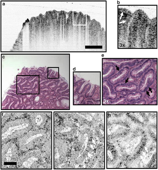
Fig. 1.22
OCT and OCM images of lower GI pathology ex vivo. (a, b) OCT of tubular adenoma shows parallel arrangement of long, slender crypt units, with the crypt epithelium identifiable from the lamina propria (b, arrows). (c–e) Corresponding histology. (f–h) OCM visualizes architecture en face, showing eccentric crypt lumens with varying shape and arrangement as well as oval-shaped nuclei. (e) Histology in the transverse plane shows corresponding features. OCM image depths for (f–h) were 80, 90, and 190 um, respectively. Scale bars: (a, c) 500 um; (f–h) 100 um (Aguirre et al. [84])
Although OCM has advantages in resolution, early OCM methods were difficult to implement because it was necessary to match the interferometer reference arm delay to the scanned beam path delay in the microscope sample arm interface. Standard confocal or multiphoton microscopes do not require constant path delay beam scanning and therefore it was difficult to make early OCM technology compatible with existing microscope designs. In addition, OCM requires acquiring one axial scan for each pixel in the image, because the image is in the en face plane. Therefore, high imaging speeds were needed in order to generate high pixel resolution images using standard OCT detection methods. Advances in OCT image speeds using spectral/Fourier domain and swept source/Fourier domain OCT (described in the next section) provided a solution to the problem of path delay matching because the dramatic increase in imaging speed enabled multiple en face depths, spanning the focal depth, to be acquired during a fast raster scan [85]. Related techniques, known as en face OCT, were developed in fields such as ophthalmology [86–88]. With the advent of high-speed imaging techniques, the low numerical aperture focusing meant that en face images at multiple depths could be generated from a single volumetric data set [89–91]. This was especially powerful in ophthalmology because it enables direct comparison with standard clinical imaging methods such as fundus photography or fluorescein angiography which image the retina in an en face plane.
The development of a technique known as full-field optical coherence tomography enabled optimized en face plane imaging and achieved extremely high pixel density images over wide fields of view [92–94]. Full-field OCT performs high-resolution en face imaging with coherence-gated detection using a Linnik interferometer and CCD cameras. Full-field OCT achieves cellular resolution imaging, and because a single spatial mode light is not required, it has the advantage that high axial resolution is possible using low-cost thermal or gas discharge light sources. Part II of this book, Optical Coherence Microscopy, includes several chapters which describe different approaches for en face imaging.
Stay updated, free articles. Join our Telegram channel

Full access? Get Clinical Tree


