Habit 1: Check Quality Before Quantity

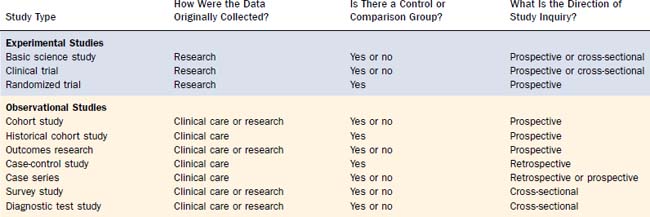
Bias is a four-letter word that is easy to ignore but difficult to avoid.⁴ Data collected specifically for research (Table 6-2) are likely to be unbiased—they reflect the true value of the attribute being measured. In contrast, data collected during routine clinical care will vary in quality depending on the specific methodology applied.

Table 6-2 Effect of Study Design on Data Interpretation

Experimental studies, such as randomized trials, often yield high-quality data because they are performed under carefully controlled conditions. In observational studies, however, the investigator is simply a bystander who records the natural course of health events during clinical care. Although more reflective of “real life” than a contrived experiment, observational studies are more prone to bias. Comparing randomized trials with outcomes studies highlights the difference between experimental and observational research (Table 6-3).

Table 6-3 Comparison of Randomized Controlled Trials and Outcomes Studies

The presence or absence of a control group has a profound influence on data interpretation. An uncontrolled study, no matter how elegant, is purely descriptive.⁵ Nonetheless, authors of case series often delight in unjustified musings on efficacy, effectiveness, association, and causality. A case series is of greatest value when dealing with uncommon disorders or interventions, or with circumstances in which randomized trials would be unethical or impractical. The best case series include a consecutive sample of subjects, describe the sample fully, include details of interventions and adjunctive treatments, account for all participants enrolled (including withdrawals and dropouts), and ensure that follow-up duration is adequate to overcome random disease fluctuations.⁶

Without a control or comparison group, treatment effects cannot be distinguished from other causes of clinical change (Table 6-4). Some of these causes are seen in Figure 6-1, which depicts change in health status after a healing encounter as a complex interaction of three primary factors^7–8:

Table 6-4 Explanations Other Than “Efficacy” for Outcomes in Treatment Studies

Figure 6-1. Model depicting change in health status after a healing encounter. Dashed arrow shows that a placebo response may occur from symbolic significance of the specific therapy given or from interpersonal aspects of the encounter.

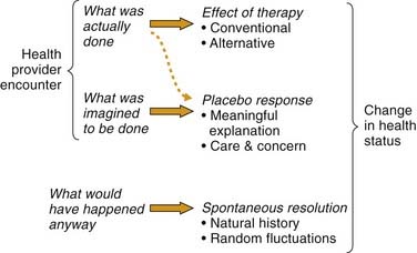
The placebo response differs from the traditional definition of placebo as an inactive medical substance. Whereas a placebo can elicit a placebo response, the latter can occur without the former. A placebo response results from the psychological or symbolic importance attributed by the patient to any nonspecific event in a healing environment. These events include touch, words, gestures, local ambience, and social interactions.¹⁰ Many of these factors are encompassed in the term caring effects,¹¹ which have been central to medical practice in all cultures throughout history. Caring and placebo effects are so important that they have been deliberately used to achieve positive outcomes in clinical practice.¹²

When data from a comparison or control group are available, inferential statistics may be used to test hypotheses and measure associations. Causality may also be assessed when the study has a time span component, either retrospective or prospective (see Table 6-2). Prospective studies measure incidence (new events) whereas retrospective studies measure prevalence (existing events). Unlike time span studies, cross-sectional inquiries measure association not causality. Examples include surveys, screening programs, and evaluation of diagnostic tests. Experimentally planned interventions are ideal for assessing cause-effect relationships, because observational studies are prone to innate distortions or biases caused by individual judgments and other selective decisions.¹³

Another clue to data quality is study type,¹⁴ but this cannot replace the four questions in Table 6-2. Note the variability in data quality for the study types listed in Table 6-5, particularly the observational designs. Randomization balances baseline prognostic factors (known and unknown) among groups, including severity of illness and the presence of comorbid conditions. Because these factors also influence a clinician’s decision to offer treatment, nonrandomized studies are prone to allocation (susceptibility) bias (see Table 6-3) and false-positive results.¹⁵ For example, when the survival of surgically treated cancer patients is compared with the survival of nonsurgical controls (e.g., radiation or chemotherapy), without randomization, the surgical group will generally have a more favorable prognosis independent of therapy, because the customary criteria for operability (special anatomic conditions and no major comorbidity) also predispose to favorable results.

Table 6-5 Relationship of Study Type to Study Methodology

The relationship between data quality and interpretation is illustrated in Table 6-6 using hypothetical studies to determine whether tonsillectomy causes baldness. Note how a case series (examples 1 and 2) can have either a prospective or retrospective direction of inquiry depending on how subjects are identified; contrary to common usage, all cases series are not “retrospective reviews.” Only the controlled studies (examples 3 through 7) can measure associations, and only the controlled studies with a time span component (examples 4 through 7) can assess causality. The nonrandomized studies (examples 3 through 6), however, require adjustment for potential confounding variables—baseline prognostic factors that may be associated with both tonsillectomy and baldness and therefore influence results. As noted previously, adequate randomization ensures balanced allocation of prognostic factors among groups, thereby avoiding the issue of confounding.

Table 6-6 Determining If Tonsillectomy Causes Baldness: Study Design vs. Interpretation

* Studies are listed in order of increasing ability to establish causal relationship.

Habit 2: Describe Before You Analyze

Statistical tests often make assumptions about the underlying data. Unless these assumptions are met, the test will be invalid. Describing before you analyze avoids trying to unlock the mysteries of square data with a round key.

Describing data begins by defining the measurement scale that best suits the observations. Categorical (qualitative) observations fall into one or more categories and include dichotomous, nominal, and ordinal scales (Table 6-7). Numerical (quantitative) observations are measured on a continuous scale and are further classified by the underlying frequency distribution (plot of observed values vs. the frequency of each value). Numerical data with a symmetric (normal) distribution are symmetrically placed around a central crest or trough (bell-shaped curve). Numerical data with an asymmetric distribution are skewed (shifted) to one side of the center, have a sloping “exponential” shape that resembles a forward or backward J, or contain some unusually high or low outlier values.

Table 6-7 Measurement Scales for Describing and Analyzing Data

Depending on the measurement scale, data may be summarized using one or more of the descriptive statistics in Table 6-8. Note that when summarizing numerical data, the descriptive method varies according to the underlying distribution. Numerical data with a symmetric distribution are best summarized with the mean and standard deviation (SD), because 68% of the observations fall within the mean ± 1 SD and 95% fall within the mean ± 2 SD. In contrast, asymmetric numerical data are best summarized with the median, because even a single outlier can strongly influence the mean. If a series of five patients are followed after sinus surgery for 10, 12, 15, 16, and 48 months, the mean duration of follow-up is 20 months, but the median is only 15 months. In this case a single outlier, 48 months, distorts the mean.

Table 6-8 Descriptive Statistics

* Also called the absolute risk reduction.

Although the mean is appropriate only for numerical data with a symmetric distribution, it is often applied regardless of the underlying symmetry. An easy way to determine whether the mean or median is appropriate for numerical data is to calculate both; if they differ significantly, the median should be used. Another way is to examine the SD; when it is very large (e.g., larger than the mean value with which it is associated), the data often have an asymmetric distribution and should be described by the median and interquartile range. When in doubt, the median should always be used over the mean.¹⁶

A special form of numerical data is called censored (see Table 6-7). Data are censored when three conditions apply: (1) the direction of study inquiry is prospective, (2) the outcome of interest is time-related, and (3) some subjects die, are lost, or have not yet had the outcome of interest when the study ends. Interpreting censored data is called survival analysis, because of its use in cancer studies where survival is the outcome of interest. Survival analysis permits full use of censored observations by including them in the analysis up to the time the censoring occurred. If censored observations are instead excluded from analysis (e.g., exclude all patients with less than 3 years of follow-up in a cancer study), the resulting survival rates will be biased and sample size will be unnecessarily reduced.

A survival curve starts with 100% of the study sample alive and shows the percentage still surviving at successive times for as long as information is available. The curve may be applied not only to survival as such, but also to the persistence of freedom from a disease or complication or some other end point. For example, one could estimate the 3-year, 5-year, or 10-year rates for cholesteatoma recurrence or the future “survival” of tonsils (e.g., no need for tonsillectomy) in a cohort of children after adenoidectomy alone. Several statistical methods are available for analyzing survival data. The Kaplan-Meier (product-limit) method records events by exact dates and is suitable for small and large samples. Conversely, the life table (actuarial) method records events by time interval (e.g., every month, every year) and is most commonly used for large samples in epidemiologic studies.

The odds ratio, relative risk, and rate difference (see Table 6-7) are useful ways of comparing two groups of dichotomous data.¹⁷ A retrospective (case-control) study of tonsillectomy and baldness might report an odds ratio of 1.6, indicating that bald subjects were 1.6 times more likely to have had tonsillectomy than were nonbald controls. In contrast, a prospective study would report results using relative risk. A relative risk of 1.6 means that baldness was 1.6 times more likely to develop in tonsillectomy subjects than in nonsurgical controls. Finally, a rate difference of 30% in a prospective trial or experiment reflects the increase in baldness caused by tonsillectomy, above and beyond what occurred in controls. No association exists between groups when the rate difference equals zero, or the odds ratio or relative risk equals one (unity).

Two groups of ordinal or numerical data are compared with a correlation coefficient (see Table 6-8). A coefficient (r) from 0 to 0.25 indicates little or no relationship, from 0.25 to 0.49 a fair relationship, from 0.50 to 0.74 a moderate to good relationship, and greater than 0.75 a good to excellent relationship. A perfect linear relationship would yield a coefficient of 1.00. When one variable varies directly with the other, the coefficient is positive; a negative coefficient implies an inverse association. Sometimes the correlation coefficient is squared (r²) to form the coefficient of determination, which estimates the percentage of variability in one measure that is predicted by the other.

Habit 3: Accept the Uncertainty of All Data

Uncertainty is present in all data, because of the inherent variability in biologic systems and in our ability to assess them in a reproducible fashion.¹⁸ If hearing in 20 healthy volunteers was measured on five different days, how likely would it be to get the same mean result each time? It is very unlikely, because audiometry has a variable behavioral component that depends on the subject’s response to a stimulus and the examiner’s perception of that response. Similarly, if hearing was measured in five groups of 20 healthy volunteers each, how likely would it be to get the same mean hearing level in each group? Again unlikely, because of variations between individuals. A range of similar results would be obtained, but rarely the exact same result on repetitive trials.

Uncertainty must be dealt with when interpreting data, unless the results are meant to apply only to the particular group of patients, animals, cell cultures, and DNA strands, in which the observations were initially made. Recognizing this uncertainty, each of the descriptive measures in Table 6-8 is called a point estimate, specific to the data that generated it. In medicine, however, one seeks to pass from observations to generalizations, from point estimates to estimates about other populations. When this process occurs with calculated degrees of uncertainty, it is called inference.

The following is a brief example of clinical inference. After treating five vertiginous patients with vitamin C, you remark to a colleague that four had excellent relief of their vertigo. She asks, “How confident are you of your results?”

“Quite confident,” you reply. “There were five patients, four got better, and that’s 80%.”

“Maybe I wasn’t clear,” she interjects, “how confident are you that 80% of vertiginous patients you see in the next few weeks will respond favorably, or that 80% of similar patients in my practice will do well with vitamin C? In other words, can you infer anything about the real effect of vitamin C on vertigo from only five patients?”

Hesitatingly you retort, “I’m pretty confident about that number 80%, but maybe I’ll have to see a few more patients to be sure.”

The real issue, of course, is that a sample of only five patients offers low precision (repeatability). How likely is it that the same results would be found if five new patients were studied? Actually, one can state with 95% confidence that four out of five successes in a single trial is consistent with a range of results from 28% to 99% in future trials. This 95% confidence interval may be calculated manually or with a statistical program; it reveals the range values considered plausible for the population. A point estimate summarizes findings for the sample, but extrapolation to the large population introduces error and uncertainty, which makes a range of plausible values more appropriate.

Precision may be increased (uncertainty may be decreased) by using a more reproducible measure, by increasing the number of observations (sample size), or by decreasing the variability among the observations. The most common method is to increase the sample size, because the variability inherent in the subjects studied can rarely be reduced. Even a huge sample of perhaps 50,000 subjects still has some degree of uncertainty, but the 95% confidence interval will be quite small. Realizing that uncertainty can never completely be avoided, statistics are used to estimate precision. Thus when data are described using the summary measures listed in Table 6-8, a corresponding 95% confidence interval should accompany each point estimate.

Precision differs from accuracy. Precision relates to random error and measures repeatability; accuracy relates to systematic error (bias) and measures nearness to the truth. A precise otologist may always perform a superb mastoidectomy, but an accurate otologist performs it on the right patient. A precise surgeon cuts on the exact center of the line, but an accurate surgeon first checks the line to be sure it is in the right place. Succinctly put, precision is doing things right and accuracy is doing the right thing. Precise data include a large enough sample of carefully measured observations to yield repeatable estimates; accurate data are measured in an unbiased manner and reflect what is truly purported to be measured. When we interpret data, we must estimate both precision and accuracy.

To summarize habits 1, 2, and 3: “Check quality before quantity” determines whether or not the data are worth interpreting (habit 1). Assuming they are, “describe before you analyze” and summarize the data using appropriate measures of central tendency, dispersion, and outcome for the particular measurement scales involved (habit 2). Next, “accept the uncertainty of all data” as noted in habit 3, and qualify the point estimates in habit 2 with 95% confidence intervals to measure precision. When precision is low (e.g., the confidence interval is wide), proceed with caution. Otherwise, proceed with habits 4, 5, and 6, which deal with errors and inference.

Habit 4: Measure Error with the Right Statistical Test

To err is human—and statistical. When comparing two or more groups of uncertain data, errors in inference are inevitable. If one concludes that the groups are different, they may actually be equivalent. If one concludes that they are the same, a true difference may have been missed. Data interpretation is an exercise in modesty, not pretense—any conclusion we reach may be wrong. The ignorant data analyst ignores the possibility of error; the savvy analyst estimates this possibility by using the right statistical test.¹⁹

Now that we’ve stated the problem in English, let’s restate it in thoroughly confusing statistical jargon (Table 6-9). We begin with some testable hypotheses about the groups we are studying, such as “Gibberish levels in group A differ from those in group B.” Rather than keep it simple, we now invert this to form a null hypothesis: “Gibberish levels in group A are equal to those in group B.” Next we fire up our personal computer, enter the gibberish levels for the subjects in both groups, choose an appropriate statistical test, and wait for the omnipotent P value to emerge.

Table 6-9 Glossary of Statistical Terms Encountered When Testing Hypotheses

Only gold members can continue reading. Log In or Register to continue

Share this:

• Click to share on Twitter (Opens in new window)
• Click to share on Facebook (Opens in new window)

Related

Related posts:

1. Laryngeal and Tracheal Manifestations of Systemic Disease
2. Nasal Reconstruction
3. Surgical Robotics in Otolaryngology
4. Malignant Tumors of the Larynx

Stay updated, free articles. Join our Telegram channel

Join

Tags: Cummings Otolaryngology - Head and Neck Surgery Head and Neck Su

Jun 5, 2016 | Posted by admin in OTOLARYNGOLOGY | Comments Off on Interpreting Medical Data

Full access? Get Clinical Tree

Get Clinical Tree app for offline access

Get Clinical Tree app for offline access

Term	Definition
Central tendency	A supposition, arrived at from observation or reflection, that leads to predictions which can be tested and refuted
Null hypothesis	Results observed in a study, experiment, or test that are no different from what might have occurred due to chance alone
Statistical test	Procedure used to reject or accept a null hypothesis; statistical tests may be parametric, nonparametric (distribution-free), or exact
Type I (alpha) error