Fig. 16.1
Common vascular features in IVOCT images
The typical speed for current IVOCT imaging is 50,000 lines/s and 100 frames/s (this is the specifications for C7-XRTM OCT Intravascular Imaging System, St. Jude Medical Inc., St. Paul, Minnesota, the current IVOCT system from Terumo Europe N.V. has higher speed, as will the next generation system from St. Jude Medical). The amount of image data and details generated by OCT can be overwhelming to the practicing clinician. Currently, analysis of OCT images has been typically conducted manually in an extremely time-consuming manner. For instance, for stent analysis, analysts need to manually mark every stent strut in a pullback. Based on our experience, it usually takes more than 7 h to analyze all the frames in a single pullback. In addition, many quantitative metrics of potential clinical diagnostic values are difficult to be generated by manual-based methods. Automated image analysis can (1) greatly alleviate the burdens of analysts, (2) provide more comprehensive metrics for diagnosis, (3) help reduce interobserver variability, and (4) be potentially used for live-time analysis during clinical procedures.
16.2 Image Display and Calibration
IVOCT images are naturally acquired in polar coordinates (Fig. 16.2). After logarithmic compression, images are typically converted from polar to Cartesian coordinates for display. Notice that due to the helical scanning pattern during imaging, the cross-sectional plane is actually oblique with respect to the pullback direction. In commercial OCT systems, longitudinal view (L-mode) image is also used. It is obtained by combining all image pixels at the plane intersects the catheter center at one rotation angle (Fig. 16.2 bottom).
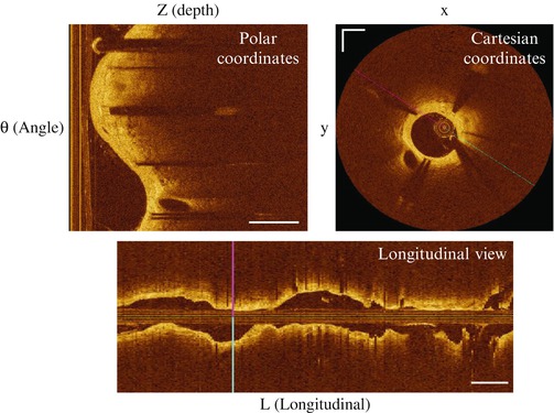

Fig. 16.2
Visualization modes of IVOCT images. Scale bar: 1 mm for the top panels; 5 mm for the bottom panel
Before any image analysis, calibration must be performed to ensure accurate measurements [12]. Calibration is performed by adjusting the z-offset, which is the optical path length of the optical fiber within the catheter. In practice, cross-sectional images in Cartesian coordinates are adjusted to match the outer boundary of the catheter with the actual diameter. In the corresponding polar coordinates, adjusting the z-offset is equivalent to translating the image in the A-line direction. As the optical path length may change during a single pullback, the z-offset often needs to be adjusted multiple times during the analysis of a single pullback.
16.3 Segmentation, Detection, and Quantification Methods
Segmentation refers to partitioning an image into meaningful regions with different labels. It is fundamental for IVOCT image analysis and is the basis for quantification, plaque characterization, recognition, and 3-D visualization. Detection is to automatically detect meaningful features (e.g., stent struts) from original images and is often the basis for tissue quantification, recognition, and 3-D visualization.
16.3.1 Lumen Segmentation
Lumen segmentation is often the basis for more advanced plaque and stent analysis. In addition, lumen area itself is a direct indicator of vessel stenosis. In OCT images, luminal boundary is very distinctive, and it is likely that many image processing techniques can succeed in this task [13–16]. We describe two methods here, and both have been proved to be robust in practice. The first one is a 2-D optimization method using dynamic programming [17, 18], and the second one is a 3-D optimization method using closure graph and graph cut [19]. Later, one can see that the basic principles of the two methods can be easily extended to other applications.
16.3.1.1 2-D Dynamic Programming Method
Searching for the vessel luminal boundary in the polar coordinates of OCT images fits the graph search family of optimization problems naturally. The lumen boundary is unique and the accumulated optical intensity difference between the pixels from the vessel and luminal side along the contour is maximum. The globally optimal boundary can be efficiently found using a classic optimization method, dynamic programming (DP).
DP is a general technique used to solve certain optimization problems [20]. The basic concept is to find the globally optimal solution to the original problem by building on optimal solutions to subproblems. It is very robust in the presence of noise, and this is attractive to OCT image analysis because OCT images often suffer from speckle noise and various artifacts. Consider the OCT images in polar coordinates (θ, r) where θ is angle and r is depth. Suppose there are m A-lines in one image. We assign each pixel at row i and column j an objective function f(i, j) favoring the characteristics of lumen boundary. Our goal is to search for a path from row 1 to row m with the optimal cost C. We can break the problem into subproblems such that the path to row i is always coming from the path to i−1 with some connectivity constraint. Therefore, we have the following recursive function:

where C(i, j) is the accumulated cost from row 1 to point (i, j), j* is adjacent to j, and n specifies connectivity. The globally optimal boundary can be found by selecting the point in row m with the maximum accumulated cost and back tracking the path [17, 18]. f(i, j) can be simply defined as the intensity difference between image pixels on the vessel side and the luminal side:

where  refers to the average of pixel value and w is the length of the window for averaging. When the guide wire stays close to the lumen boundary, its bright reflections may obscure the lumen boundary and need to be excluded from lumen segmentation. This can be achieved by guide wire segmentation introduced in Sect. 16.3.2. For image segmentation, the advantages of DP include its global optimum nature, simplicity, and stability. The limitation is that it is not easy to be generalized to 3-D or higher dimensional space.

(16.1)

(16.2)
 refers to the average of pixel value and w is the length of the window for averaging. When the guide wire stays close to the lumen boundary, its bright reflections may obscure the lumen boundary and need to be excluded from lumen segmentation. This can be achieved by guide wire segmentation introduced in Sect. 16.3.2. For image segmentation, the advantages of DP include its global optimum nature, simplicity, and stability. The limitation is that it is not easy to be generalized to 3-D or higher dimensional space.
16.3.1.2 3-D Method: Surface Segmentation Using Graph Cut
The 3-D lumen segmentation method is based on the surface segmentation method proposed by Li et al. [21]. It is worth mentioning that this method has been successfully applied to intraretinal layer segmentation in ophthalmic OCT images by Garvin et al. [22]. The main idea of the method consists of two steps [21]. First, the volumetric images are transformed into a closure graph, where the optimal closed set corresponds to the optimal surfaces in the original images. The second step is to search for the optimal closed set using graph cut algorithms. We next introduce the method.
We denote a voxel V in the IVOCT pullback as V(z, θ, l), where z, θ, l are the coordinate in the axial, lateral, and longitudinal direction, respectively. We first look at how we can transform the image stack into a closure graph according to the work by Wu et al. [23] and Li et al. [21]. Consider a directed graph G = (V, E) with nodes V and edges E. Each node is formed by a voxel in the IVOCT pullback in polar coordinates. Each node is associated with a weight c(z, θ, l) (node weight) penalizing the probability of it being located on the lumen boundary, taking the form defined in Eq. 16.2.
We denote the farthest plane from the catheter in the IVOCT pullback as the base layer (z = 0). Then, the top plane (closest to the catheter) is represented by z = N−1, where N is the number of points in each A-line. We change the node weight from c(z, θ, l) to w(z, θ, l) as follows:


(16.4)
Notice that we can incorporate the special helical scanning pattern of IVOCT into the neighborhood definition, i.e., the last A-line in frame i is adjacent to the first A-line in frame i + 1. These directed edges will be assigned infinite edge weight, and this ensures that the resulting surface intersects each A-line exactly once, and the surface is also smooth as defined by the smoothness hard constraint. In addition to the hard constraints, one can also add soft constraints between neighboring A-lines by assigning the edges finite edge weights [24, 25]. Soft constraints allow, but can penalize, the surface boundary deviating from predefined shape priors [24]. Finally, we make the base layer strongly connected (every node in this layer is reachable from any other node) by making infinite edge links between the nodes in the layer such that this layer cannot be cut. Now, one can see that the optimal surface of the original IVOCT pullback corresponds to the optimal closed set (constituted by all the nodes on and below the surface) in the graph G [21, 23].
Searching for the optimal closed set in a graph can be efficiently solved using max-flow/min-cut algorithm, as shown by Picard in the 1970s [26]. Briefly, we construct a closure graph G C from G by adding two special nodes source s and sink t. We create directed edges linking s to all the nodes with negative weights and edges connecting all nodes with positive weights to t, with the edge weight equal to the absolute value of the node weight. A cut in a graph partitions the graph into two disjoint sets containing s and t, respectively. The minimum cut is the cut where the sum of edges it severs is minimum. The minimum cut is also a finite cut and can only sever finite edges connected to s/t in G C . One can easily prove that after a finite cut, the set containing s becomes a closed set and the optimal closed set corresponds to the minimum cut of this closure graph [26, 27].
The surface segmentation method presented above is ideal for robust 3-D lumen segmentation due to its global optimum nature. However, the time and space complexity of the method is huge. For typical IVOCT image stack consisting of 500*1,000*271 pixels, it takes several hours for state-of-the-art graph algorithms to compute the optimal surface, which is impractical for real applications. We can use a simple multi-resolution approach [28] to overcome this computation burden effectively. Consider a coarse level image stack obtained by downsampling the original image stack in axial and lateral directions. As the lumen boundary is very distinct, it still remains the globally optimal boundary although some details are lost in the coarse level. Hence, we can perform graph cut to obtain the optimal surface at this coarse level and then map it back to the original fine level. We know that the true optimal surface should be close to the mapped surface. Hence, we can perform the second round graph cut on the fine level, but only consider the voxels within a narrow band around the mapped surface. This allows the total computation time to be reduced to <1 min for a whole pullback (downsample by 8).
Examples of lumen segmentation results in challenging images are shown in Fig. 16.3.


Fig. 16.3
Examples of lumen segmentation results in challenging images. Left: an image with significant luminal blood. Middle: an image showing severe stenosis. Right: an image from a stented vessel
Remark: distinction should be made between this surface segmentation method and the general graph cut method used for image segmentation proposed by Boykoy et al. [29, 30]. The major difference lies in the graph construction stage. The surface segmentation method uses closure graphs and strictly separates the nodes above the below the surface. Therefore, it is limited to terrain-like surfaces [21]. In comparison, general graph cut [29, 30] does not use closure graphs, and it allows for segmentation of contours/surfaces with arbitrary shape but typically requires user input of seed points indicating the foreground and background. Despite these differences, the same graph cut algorithm can be used in both methods. As IVOCT images are naturally acquired in polar coordinates, the surface segmentation method can guarantee an optimal terrain-like lumen surface. However, it is important to note that the general graph cut is a powerful, globally optimal N-D segmentation method, with a wide range of applications in computer vision. More details of the method can be found in [29, 30]. For state-of-the-art graph cut algorithms, please refer to [30–33].
16.3.2 Guide Wire Segmentation
We describe a guide wire segmentation method that is able to extract the globally optimal guide wire positions of all the frames in the entire pullback at once [17, 18]. Briefly, we create an en face projection image where 2-D images of the pullback are projected to 1-D curves and combined into one image (Fig. 16.4b). The regions of the guide wire shadow become a continuous dark band. Similar to lumen segmentation, an objective function of pixel value difference is applied to the two boundaries of the dark band but with different signs. DP is then applied twice to find the two boundaries. More robustly, the two coupled boundaries could also be found simultaneously using a multiple-surface segmentation technique in higher dimensions [21], or using higher-dimension DP [34], but at the expense of increased computation time. The above described method only applies to OCT pullbacks with a single guide wire. Sometimes, there could be more than one guide wire inserted in the same vessel. In such cases, the en face view image can be combined with other methods for guide wire segmentation.
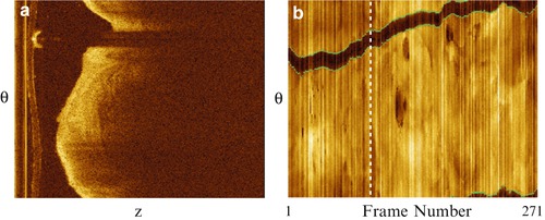

Fig. 16.4
Segmentation of guide wires using the en face projection view. (a) A cross-sectional image of a pullback showing the guide wire region with a long dark shadow. (b) The en face projection view showing the guide wire region as a continuous dark band traversing the whole pullback. The white dotted line illustrates the position of the frame (a) in the pullback. The guide wire positions of all frames can be simultaneously found by segmenting the two boundaries of the dark band. Modified from Wang et al. [17]
16.3.3 Calcified Plaque Segmentation
16.3.3.1 Level Set Segmentation Method
Level set is a popular method used for image segmentation [35–37]. It tracks the object boundaries by minimizing an appropriately designed energy function on a continuous grid using partial differential equations. Instead of explicitly representing the evolving contours using parametric models like snakes [38], level set implicitly represents a contour using the zero level set of a higher dimension function and can treat topological changes such as contour break and merge easily. We define ϕ(t, x, y) (to simplify description, we use a 2-D grid, but level set can be easily generalized to higher dimensions) as the level set function in a higher dimension, and the zero level set C = {(x, y)|ϕ = 0} represents the evolving contour. Image segmentation using level sets begins with an initial contour and then evolves it in the normal direction based on the following general equation:

where F is a speed function and is related to the image data.

(16.5)
For calcified plaque (CP) segmentation, we describe a level set approach combining the work of Li et al. [39] and Chan and Vese [40]. We define ϕ as a signed distance function (SDF) with its zero level curve represented by C. ϕ < 0 if ϕ is outside C; ϕ > 0 if ϕ is inside C. The initial contour C 0 is driven to the desired CP boundary by minimizing the following energy term:


(16.6)
δ(ϕ) is a 2-D smoothed Dirac function; H is the Heaviside function; I 0 is the original image; and g′ = 1/(1 + g), where g is the gradient image which is determined by convolving the original image with different orientations of edge filters and selecting the maximum response for each point [41]. c 1 is the average intensity inside C; c 2 is the average intensity of an outer ring of thickness w surrounding C, μ, λ, ν; and κ are weighting terms. The first term is to keep ϕ as a SDF. The second term is a length term regulating the smoothness of the contour. The third term is an area term indicating whether the curve will grow or shrink. In our implementation, it was set positive to shrink the contour. The fourth term contains region-based intensity information. The minimization of E is based on the following gradient flow:


(16.7)
The evolving contour is stopped if its speed is close to zero. In the discrete image space, all the terms in the above equations are numerically approximated. More details of the method can be found in [41]. The advantage of the level set method is its flexible topology for contour merge and break. The limitation is that it may find a local minimum instead of a global minimum. Therefore, the initial contour is often required to be placed close to the desired boundaries. Examples of automated CP segmentation results with comparison with human analysts are shown in Fig. 16.5. More details about level sets can be found in [35–37, 42].
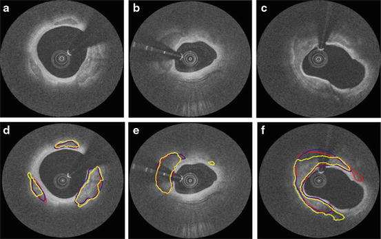

Fig. 16.5
Examples of calcified plaque segmentation results. (a–c) Original images. (d–f) Corresponding manual and automatic segmentation results. Red: observer 1; blue: observer 2; yellow: automatic method. Reprinted from Wang et al. [41]
16.3.3.2 Calcified Plaque Quantification
Based on the segmentation, the depth, area, volume, thickness, and angle fill fraction (AFF) of CP can be calculated automatically. The calculation of area is trivial. The volume of a lesion can be calculated from CP areas in individual frames using Simpson’s rule. For depth and thickness, we typically use the rays radiating from the centroid of the lumen as the direction for calculation. AFF is simply the largest angle between the rays spanned across the CP [41].
16.3.4 Fibrous Cap Quantification
The conventional method to assess the fibrous cap (FC) thickness is to quantify only the minimum cap thickness (MCT). However, as FC is a 3-D structure, the single-point/single-frame representation is unable to capture the volumetric profile of FC. In addition, we have found that significant interobserver variations exist between different analysts in assessing the MCT [17]. Here, we describe a method that is able to quantify the volumetric morphology of FC and also the conventional MCT more accurately. In this method, users first select the circumferential boundaries (start and end angle) of FC, and the algorithm automatically determines the optimal FC boundaries in the radial dimension. Quantitative metrics can then be derived from the FC segmentation.
16.3.4.1 Fibrous Cap Segmentation
FC is delineated by a luminal boundary and an abluminal boundary. The luminal boundary coincides with the vessel lumen contour. The abluminal boundary is commonly described as the “diffuse border” created by the interface between the FC and the underlying lipid pool. In the polar coordinates, searching for the FC abluminal boundary can be treated as a similar graph search problem as lumen segmentation, but with different objective function. Essentially, the goal is to design an objective function such that its optimal value corresponds to the optimal boundary that best separates the FC from the underlying lipid plaque. The FC has been defined histologically as a distinct layer of connective tissue covering the lipid core and consists purely of smooth muscle cells in a collagenous-proteoglycan matrix, with varying degrees of infiltration by macrophages and lymphocytes [43]. The fibrous tissue appears bright by OCT and has a low attenuation coefficient, whereas the lipid pool appears dark and strongly attenuates the light [44, 45]. Therefore, the FC abluminal boundary has a high intensity difference between the FC and lipid pool and also a high gradient. Hence, we define the following objective function:

where d l and d max are predefined depths to calculate pixel intensity difference, μ is the slope of pixel value attenuation extracted from the A-line segment of length L across (i, j), and λ is a weighting term. The parameter values d l = 75 μm, d max = 0.38 mm, λ = 7 and L = 38 μm are determined experimentally using training data [17]. With this objective function, the optimal FC abluminal boundary can be obtained using the same DP algorithm (Sect. 16.3.1) in the region bounded by the luminal boundary and d max in the radial dimension and by the user-selected angle in the circumferential direction. Automation of the angle selection is possible but is presently hindered by the lack of a validated, reproducible criterion for FC circumferential boundaries.

(16.8)
16.3.4.2 Quantification and 3-D Visualization
With the fully segmented FC, we can quantify the thickness at each point of the FC luminal boundary, defined as the minimum distance from this point to the FC abluminal boundary. The conventional metric MCT can be accurately found from the pool of the thicknesses of all the points. In addition, volumetric metrics of the FC can be derived. The FC surface area (SA) of a lesion can be calculated as the product of the frame interval and the arc length of FC summed over involved frames. The absolute and fractional FC categorical surface area (ACSA and FCSA) of a lesion can be calculated as the absolute and relative FC area in a thickness category (e.g., <65 μm, 65–150 μm, and >150 μm). Other possible volumetric metrics can also be found in [17].
The segmented FC can be visualized in 3-D with a continuous color map indicating the FC thickness. Figure 16.6 illustrates two cases, both with TCFA, with FC thickness rendered in 3-D. If assessed using only the conventional methodology, the morphological differences between the cases would not be apparent. However, the 3-D visualization demonstrates dramatically different characteristics.
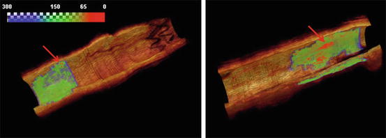

Fig. 16.6
Two coronary arteries used in the validation study with fibrous caps (FC) rendered in a continuous color map indicating the thickness. Both of the two lesions contain TCFA (red arrows) and similar minimum cap thickness. However, the plaque shown on the right panel contains a significantly larger surface area with thin cap as compared to the plaque in the left panel. Reprinted from Wang et al. [17]
16.3.5 Stent Detection
Stent analysis is one of the most common tasks for IVOCT image analysis. Several automated stent detection methods have been reported [14–16, 46–49]. Due to space constraint, we describe one method that has the advantage of having few empirical parameters and that has been validated using a large clinical dataset [50]. The method consists of two major steps, (1) probabilistic detection of strut positions and (2) simultaneous localization of all strut depths.
16.3.5.1 Probabilistic Detection of Strut Positions
As the metallic stent strongly reflects light, the struts cast clear shadows in intersecting A-lines. In comparison, surrounding tissues not covered by stents are free of strut shadows. Therefore, strut locations typically appear as extreme points in the 1-D projection, which is generated by taking the mean intensity of a fixed depth (1.5 mm) from the luminal boundary (Fig. 16.7).
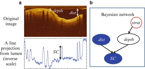

Fig. 16.7
The Bayesian network for inference of strut presence. (a) Top: original OCT image in polar coordinate. Bottom: by calculating the mean intensity of the A-line within a fixed depth from the lumen boundary, the 2-D image is projected into a 1-D curve (plotted in an inverse scale). Searching for strut locations is equivalent to searching for peaks in the 1-D curve. (b) A Bayesian network representation based on principles of OCT image formation
We consider physical principles in the detection of struts in the 1-D projection curve. If we define the relative difference between the adjacent extreme peak and valley points to be shadow contrast (SC), it can be seen that real struts generate larger SC as compared to surrounding non-strut regions, but the size of SC depends on how far the lumen wall is from the catheter (represented by dist) and how deep the tissue is covering the strut (represented by depth). We can model these cause-effect relationships using a Bayesian network [51–53] as shown in Fig. 16.7b. It encodes the causal dependencies between variables and, more importantly, compactly represents the full joint probability distribution of the atomic event defined by all the variables. For example, the node SC encodes the conditional probability P(SC|dist,depth), i.e., probability of SC being a certain value given the observed values of dist and depth. For baseline cases where the OCT is performed immediately after stent implantation, the network can be simplified by not considering the strut depth.
In the stent detection problem defined in Fig. 16.7, our task is to query the probability of strut presence among all the peaks given our observations. Here, we can directly observe the values of SC and dist. We can also estimate the probabilities of P(strut) and P(SC|dist,depth) from manually analyzed training data. As SC, dist, and depth are continuous variables, we can discretize them into bins to generate the conditional probability tables (for depth, we include an additional variable, undefined, to make it compatible with presence of no strut). Note that the strut depth is still unknown at this point. According to probability theory, we can directly query P(strut|SC,dist) by marginally summing over all the possible depths a strut could occupy:


