Doppler Fourier Domain Optical Coherence Tomography for Label-Free Tissue Angiography

Fig. 42.1

Classification of methods for DOCT and optical angiography

42.3 Theory

42.3.1 Phase-Sensitive DOCT

In Fourier domain optical coherence tomography (FDOCT), the Fourier transformation of the spectral interferometric fringe signal measured by a single exposure of the line scan light detector creates one line of a structural cross-sectional image (A-scan). In order to assess the velocity of a moving interface, most known methods require at least two spectral fringes acquired at the same or nearly the same lateral position [17, 69] of a sampling light beam. This allows the calculation of the initial phase difference between the two spectral fringe signals; this difference is directly linked to the optical path change between the reference mirror and a moving reflecting or scattering object within the sample. In general, a higher number of spectra can be acquired over time to increase the accuracy of the velocity estimation. The acquired set of spectral fringes can be described as a function of the wavenumber k and time t according to the following equation:

$I\left(k,t\right)={I}_0(k)\left({\displaystyle \sum_l{R}_l}+{R}_r+2{\displaystyle \sum_l\sqrt{R_l{R}_r} \cos \left(2{z}_l(t)\cdot k\right)}\right),$

(42.1)

where I(k, t) is the spectral fringe signal; I ₀(k) is the spectral density of the light source; R _land R _rdenote the reflectivity of the sample and reference mirrors, respectively; and z _l(t) denotes the optical path difference between the reference mirror and the l–th interface in the sample. The optical path difference is time dependent due to the movement of the reference mirror and/or the displacement of the interfaces within the sample. This displacement is caused either by the movement of the entire sample or of the specific interface z _lwithin the sample. If we assume that both the reference mirror velocity and the velocities in the sample are constant during the acquisition of the spectral fringes, see Eq. 42.1, then the time-dependent position of the l–th interface, z _l(t), can be expressed as:

${z}_l(t)={z}_l+\delta z(t)={z}_l+{v}_l\cdot t.$

(42.2)

In this relation, z _lis the depth position of the l–th interface when data acquisition begins, and v _lis the difference between the velocity of the reference mirror and an axial component of the velocity of the l–th interface (parallel to the direction of the probing beam propagation). One can rewrite Eq. 42.1 making use of Eq. 42.2:

$I\left(k,t\right)={I}_0(k)\left({\displaystyle \sum_l{R}_l}+{R}_r+2{\displaystyle \sum_l\sqrt{R_l{R}_r} \cos \left(2\left({z}_l+\Delta {z}_l(t)\right)\cdot k\right)}\right)$

(42.3)

$I\left(k,t\right)={I}_0(k)\left({\displaystyle \sum_l{R}_l}+{R}_r+2{\displaystyle \sum_l\sqrt{R_l{R}_r} \cos \left(2{z}_l\cdot k+{\omega}_l\cdot t\right)}\right)$

(42.4)

Although the above equations represent the same interference pattern, they emphasize different properties. The phase of the oscillatory component present in Eq. 42.3 is a function of the wavenumber, and its modulation frequency depends on the static position z _lof the l–th interface, and a small additional change δz that occurs if the l–th interface is moving. Equation 42.4 highlights the time dependence of the interferometric fringes and shows that the signal is modulated in time with frequency ω _l. This beat frequency is caused by a Doppler effect that arises for each l–th interface along the time axis. The frequency depends on the velocity v _land is different for each wavenumber k:

${\omega}_l=2{v}_lk$

(42.5)

The phase-resolved methods [17] for estimating velocity use the signals’ phase differences as described by Eqs. 42.3 and 42.5:

${v}_l=\frac{{\Delta \Phi}_l}{2k\Delta t}=\frac{\lambda }{4\Delta t}\frac{\Delta \Phi}{\pi }$

(42.6)

Here, ΔΦ is the phase difference between successively recorded depth profiles at the same location of the probing beam:

${\Delta \Phi}_l=2\Delta {z}_lk=2{v}_l\Delta tk,$

(42.7)

The time between the acquisitions of successive profiles, Δt, is approximately equal to the exposure time of the detector; therefore, 1/Δt is the frame rate of an array detector (or equivalently, the “A-scan” rate). It is important to ensure that |ΔΦ| is less than π.

42.3.2 Optical Angiography

In the following chapter, we will focus on the DOCT modalities for noninvasive tissue angiography. In general, all methods can be realized with either spectrometer-based FdOCT or swept source OCT (SSOCT). SSOCT has particular advantages for motion sensing as it does not suffer from fringe washout and keeps high sensitivity even for several hundred kHz A-scan rates, due to its higher dynamic range than CCD or CMOS-based FdOCT and the option of dual-balanced detection. In the present chapter, we would like to demonstrate applications of tissue angiography in ophthalmology and dermatology. Those have been obtained with intensity-based DOCT, which is well adapted to swept source OCT, because it is independent from any acquisition timing problems such as trigger jitter. Also the fact that it does not require bulk motion correction alleviates the post-processing effort as compared to other techniques. An angiographic image volume P(x, y, z), contrasting flow against static tissue, is obtained by calculating the squared intensity difference between successive tomograms [35]:

$P\left(x,{y}_i,z\right)={\left(I\left(x,{y}_i,z\right)-I\left(x,{y}_{i+1},z\right)\right)}^2,$

(42.8)

where I(x, y, z) = 20 ⋅ log[FFT(I(x, y, k))], (x, y, z) are the spatial pixel coordinates corresponding to fast and slow scanning and depth coordinate, respectively, and k is the wavenumber. Such method requires good correlation for static tissue over successive tomograms. This is obtained by driving the slow axis scanner with a multiple-step function. It allows for measuring N tomograms at the same position y. A calculation of the intensity squared difference mean value at each position permits to detect decorrelation, caused by motion artifact, and to potentially reject that picture for further processing by setting manually a threshold T. The value of T is chosen such as to obtain visually optimal vessel contrast. The pictures representing the same location can be averaged to increase SNR. The number of pictures averaged at each position can be formally written as:

$M(y)={\displaystyle \sum_{i=0}^{N-1}\left(\left[{\displaystyle \sum_{x,z}P\left(x,{y}_i,z\right)}\right]<T\right)}.$

(42.9)

The logic operation in the brackets yields 1 or 0 for TRUE or FALSE, respectively. Finally, the motion contrast volume V is obtained by averaging only over the remaining M intensity squared difference tomograms P:

$V\left(x,y,z\right)=\frac{1}{M(y)}{\displaystyle \sum_{i=0}^{N-1}\left(\left[{\displaystyle \sum_{x,z}P\left(x,{y}_i,z\right)}\right]<T\right)}\cdot P\left(x,{y}_i,z\right).$

(42.10)

This method is more robust against motion artifacts than a variance analysis over the full tomogram series acquired at the same position, since pictures with strong decorrelation are rejected. Furthermore, the difference is only calculated between successive tomograms, thus reducing the time interval over which correlation is required. This improves further the stability with respect to motion artifacts.

In principle, one could replace the intensity difference in Eq. 42.8 by the difference of the full complex signal or by the phase difference only. The phase has the advantage of being insensitive to changing backscattering intensity. To be precise, the phase noise will scale with the SNR as is outlined also in the next chapter. Phase-sensitive contrasting of flowing blood seems to perform also better in case of strongly scattering embedding tissue, whereas intensity-based techniques are particularly well suited in case the embedding tissue scatters less than blood. Using the full complex signal is therefore a good compromise.

42.3.3 Noise in DOCT

In view of the importance of phase, it is therefore worth investigating the factors that determine phase fluctuations. In a scanning OCT system, phase fluctuations have two to three contributions [2] depending on the modality. Shot noise causes phase fluctuations that depend on the SNR as $\Delta {\varphi}_{SNR}=1/\sqrt{SNR}$ . In the case of shot noise limited detection the distributions of the OCT signal phase and amplitude can be found using the formalism presented by Goodman [36].

The probability density function for the phase can be described by the following expression:

$p\left(\Phi \right)=\left\{\begin{array}{cc}\hfill \frac{e^{-{\kappa_{zt}}^2/2}}{2\pi }+\frac{\kappa_{zt} \cos \Phi}{\sqrt{2\pi }} \exp \left[-\frac{{\kappa_{zt}}^2{ \sin}^2\Phi}{2}\right]\Omega \left({\kappa}_{zt} \cos \Phi \right)\hfill & \hfill - \pi <\Phi \le \pi \hfill \\ {}\hfill 0\hfill & \hfill \mathrm{otherwise}\hfill \end{array}\right.,$

(42.11)

where function $\Omega (b)=\frac{1}{\sqrt{2\pi }}{\displaystyle \underset{-\infty }{\overset{b}{\int }}{e}^{-{y}^2/2}\mathrm{d}y}$ , κ _zt= s _zt/σ is the signal-to-noise ratio (SNR) of the OCT signal dependent on time, s _ztis the amplitude of the signal, and σ is the standard deviation of the noise in the real and imaginary parts of the complex-valued time-dependent A-scans. With increasing κ _zt, the density function narrows, and it converges toward a Dirac delta function centered at Φ = 0. When the signal s decreases to zero (κ _zt→ 0), the distribution converges to a uniform distribution as seen in Fig. 42.2a. Since the phase-resolved FdOCT requires phase subtraction, the width of the final distribution becomes broader. As the distribution broadens, more random wrapped phase differences are detected, and in turn, the averaged value of the phase differences moves closer to zero.

Fig. 42.2

(a) Phase distributions for various values of the κ _ztparameter. (b) The probability density functions for the amplitude at different values of parameter κ _zω. The black curve corresponds to the distributions of amplitude for pure noise (κ_zω = 0), and the red curve is for a signal with a critical value (κ _zω= 7) that assures the correct recovery of the velocity in DOCT [36]

The probability density function of the amplitude of a time-dependent OCT signal is given by a Rician density function:

$$$ p(a)=\left\{\begin{array}{cc}\hfill \frac{a}{\sigma^2} \exp \left[-\frac{a^2+{s_{z\omega}}^2}{2{\sigma}^2}\right]{I}_0\left(\frac{a{s}_{z\omega }}{\sigma^2}\right)\hfill & \hfill a>0\hfill \\ {}\hfill \begin{array}{l}\\ {}0\end{array}\hfill & \hfill \begin{array}{l}\\ {}\mathrm{otherwise}\end{array}\hfill \end{array}\right., $$ ” src=”/wp-content/uploads/2017/03/A76297_2_En_43_Chapter_Equ12.gif”></DIV></DIV> <DIV class=EquationNumber>(42.12)</DIV></DIV>Where I 0(⋅) is a modified Bessel function of the first kind and zeroth order, κ zω = s zω /σ is the SNR of time-dependent A-scan, s zω is the amplitude of the signal, and σ is the standard deviation of the noise in the real and imaginary parts of the complex-valued time-dependent A-scan. As the signal s zω increases, the shape of the density function p A (a) changes from that of a Rayleigh density to approximately that of a Gaussian density with a mean equal to s zω , as shown in Fig. <A href=$ 42.2b. Due to the Fourier transform linking the time-dependent interferometric fringe signal with optical frequency-dependent one, the signal-to-noise ratio is increased for the latter ${\kappa}_{z\omega }=\sqrt{M}{\kappa}_{zt}$ , where M is the number of spectra being transformed.

Another factor influencing accuracy of DOCT is lateral scanning across a scattering surface. This gives rise to another contribution that depends on the lateral sampling according to $\Delta {\varphi}_{scan}=\sqrt{\left(4\pi /3\right)\left(1- \exp \left(-2{\left(\Delta x/d\right)}^2\right)\right)}$ where d is the 1/e² is the Gaussian beam waist in the focus, and Δx is the lateral displacement between successive A-scans [2]. The quotient d/Δx defines the lateral oversampling (Fig. 42.3). The third contribution in SSOCT systems is trigger jitter for starting an A-scan, or B-scan, depending on the post-processing scheme [37]. Any time offset of the A-scan or B-scan causes increasing phase error in depth, as the associated fringe period becomes smaller. This can be avoided by fast and precise phase-locked loops (PLL) or by cutting A-scans in post-processing.

Fig. 42.3

Phase noise depending on lateral displacement and SNR

In most cases, the phase fluctuation due to scanning across a scattering sample is most critical and dominating. Nevertheless, by increasing the lateral oversampling factor one eventually hits the boundary set by SNR (Fig. 42.3). Phase noise determines the lower boundaries of phase-sensitive methods, in particular the minimum resolvable or contrastable speed in Doppler OCT.

For a given phase noise, the minimal resolvable velocity is determined as

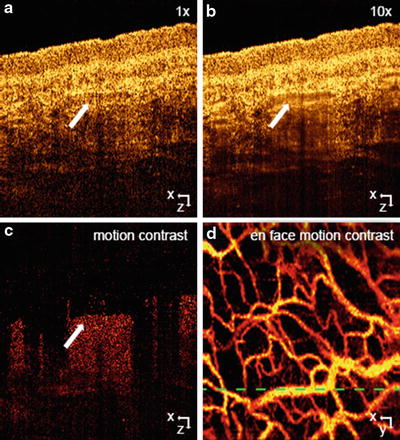
${v}_{min}=\raisebox{1ex}{$\lambda $}\!\left/ \!\raisebox{-1ex}{$4\pi T$}\right.\Delta {\varphi}_{noise}.$

(42.13)

Apart from the dependence on the phase noise, it also depends on the time interval between the signals that are used for velocity analysis. Higher sensitivity can thus be achieved by using long time intervals. If one increases the A-scan period time, the total measurement time will increase, which results in strong motion artifacts. Using two B-scans immediately allows for larger time intervals and hence higher velocity sensitivities without sacrificing total recording time. For the first time, it was possible to contrast tissue capillaries with great detail. Modern DOCT angiography techniques measure the signal decorrelation due to flow. This needs long time intervals and even higher sensitivities in order to achieve an optimal effect also for small capillaries. The high sensitivity to optical path length changes comes however at a price: flowing blood gives rise to signal decorrelation shadows below vessels. This is seen in Fig. 42.4b. Those artifacts can be reduced by weighting or even masking the vascular contrast image with the intensity image or a binarized intensity image, respectively. Those artifacts might be problematic for studying axial vasculature. They are not visible in fundus projections of DOCT angiography images. In Fig. 42.4a, another typical artifact of B-scan-based techniques is visible: horizontal stripes. They are due to increased variance or difference values in the presence of motion artifacts. They can be reduced by using a thresholding procedure as outlined in the previous chapter and by applying Fourier band-pass filtering along the direction normal to the B-scans.

Fig. 42.4

Amplitude speckle decorrelation for blood flow imaging in skin. (a) Skin tomogram, (b) average of ten tomograms taken at the same lateral location with reduce speckle contrast at the vessel location (white arrow), (c) amplitude squared difference resolving motion in red against static tissue in black, (d) en-face mean projection of the motion data set. Green dashed line indicates the position of the (a), (b), and (c)

42.3.4 Joint Spectral and Time Domain OCT

Another approach for extracting the velocity is to use the Fourier transform to detect the time-dependent frequency of the signal given in Eq. 42.4. This idea underlies the joint spectral and time domain OCT technique (STdOCT), [31] as it uses only Fourier transforms to analyze the data in the wavenumber and time domains simultaneously.

To explain the principle of the technique, it is convenient to present the data processing on a so-called STdOCT diagram (Fig. 42.5). Each of the diagram’s four panels present data connected via Fourier transforms. The transition in the horizontal direction transforms the data from the wavenumber domain to an in-depth position domain, while the vertical transitions transform the data from the time domain to the Doppler frequency domain.

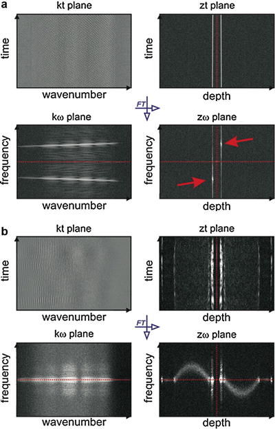
Fig. 42.5

STdOCT diagrams. Vertical transitions are accomplished by a Fourier transform along the wavenumber axis and horizontal transitions by a Fourier transform along the time axis. The amplitude of the complex signal is displayed for visualization purposes. In the zω-domain, complex conjugate images are symmetrical with respect to the central point of the plot (zero position, zero velocity). (a) Moving mirror experiment in which two points (red arrows) represent two complex conjugate images of the mirror; each of the points gives simultaneously information about the position and velocity of the moving mirror with respect to the reference mirror. (b) Laminar flow of intralipid solution in a glass capillary. Two complex conjugate images of a parabolic flow distribution are visible [65]

Two STdOCT diagrams are shown in Fig. 42.5. Figure 42.5a shows a diagram for the data acquired in a simple OCT experiment where a mirror is driven with a constant speed, and Fig. 42.5b shows a diagram for data obtained from imaging a laminar flow in a glass capillary phantom. Here, we discuss the data visible on all of the panels of the diagram.

k–t plane. Rows of the interferogram presented in this panel are simply interferometric spectra acquired by the FdOCT device that underwent standard FdOCT preprocessing (consisting of background removal, resampling to the wavenumber domain, and dispersion compensation [38]). The number of spectra is equal to the number desired to create one line of the final tomogram.

z–t plane. Data in this panel are obtained by a Fourier transform of each row from the k-t plane. Each complex-valued row in this data set is a so-called optical A-scan. Standard FdOCT processing uses these A-scans to find a line of the structural tomogram by averaging the amplitudes of the A-scans or by using phase differences between consecutive A-scans to find the Doppler shift as shown in Eq. 42.6. The signal in this plane is symmetrical with respect to the zero path delay (marked by the red dotted line).

k–ω plane. Data in this panel are obtained by Fourier transforming the data in the k-t panel with respect to time. It can be seen from Eq. 42.4 that information about the depth position of the scatterer is encoded only in the non-time-dependent component of the spectral fringe phase. Therefore, the time-dependent Fourier transform does not provide information about the in-depth localization of scatterers. However, it does provide information about the distribution of Doppler frequencies as a function of wavenumber. For the moving mirror experiment, when there is only one component in such a spectrum, its velocity can be recovered from the Doppler frequency ω _laccording to Eq. 42.5. For each k, the velocity can be calculated separately. Therefore, this representation of the data can be used to find the exact relationship between the wavenumbers and pixels in an array detector and can also be used to very accurately calibrate the spectrometer. This idea was proposed by Szkulmowski et al. [31] and discussed in detail by Faber and van Leeuwen [39]. For more complicated sample structures, it can be difficult to extract any useful information, but it is possible to filter the data to remove any undesired components of the Doppler spectrum before further processing. The optical microangiography (OMAG) technique [30] used to quantitatively visualize capillary networks uses a similar idea. The signal in this plane is symmetrical with respect to the zero velocity (marked by the red dotted line).

z–ω plane. This panel shows the result of a two-dimensional Fourier transform of the set of M spectral fringes. The coordinates of the displayed signals link the positions of all measured interfaces with their corresponding velocities. Each interface z _lis represented by two symmetrical points appearing with respect to the zero path delay and zero velocity. The sign of the velocity indicates a forward or backward direction. The point localized symmetrically with respect to the zero delay and zero velocity is the complex conjugate image of the scattering particle. The data in this panel can be regarded as a distribution of the Doppler spectrum of the signal as a function of depth, and as such, there is equivalence of the techniques developed for the time domain OCT [40–42]. It has been shown that the spread of the Doppler spectrum along the ω – axis depends on the optical parameters of the setup, such as the numerical aperture of the imaging objective, the spectral width of the light source, and the axial and transversal velocities of the imaged scattering particles. This Doppler distribution is visible in images of laminar flow as presented in Fig. 42.5b, where the distribution along the frequency axis is broadened in the center of the capillary lumen where the velocity components have their highest values in both the axial and transverse directions.

There are two ways to estimate the value of velocity component along the direction of beam propagation (Doppler component) using the STdOCT technique: maximum projection approach [31] and center of gravity approach [43]. In the first method, the velocity value is measured by finding the signal with maximum amplitude. This approach was proposed in the initial work by Szkulmowski et al. [31]. In 2011, Walther et al. [43] proposed alternative way of velocity estimation by calculating the center of gravity of the Doppler spectrum. Since the detectable Doppler frequencies are limited to half of the OCT sampling frequency, the center of gravity is calculated as the mean value of a circular distribution of amplitude. This is achieved by weighting the amplitudes by complex vectors with phases equally distributed from 0 to 2π.

${\Psi}_l\left(\kern0.15em ,{f}_D\right)={B}_l\left(\kern0.15em ,{f}_D\right)\cdot \exp \left[-i\frac{2\pi l}{N}\right]\kern0.5em \mathrm{with}\kern0.62em l=1,2,\dots, N$

(42.14)

Here, N is the number of A-scans, and B _l(f _D) is the amplitude of the l–th point Doppler frequency distribution. Finally, the center of gravity is calculated by averaging the modified complex value Ψ_l(f _D) and determining the argument for each depth z as shown in Eq. 42.15, where f _Dis the read-out rate for a single interference spectrum:

${f}_{\kern-0.2em D}(z)= \arg \left\{\frac{1}{N}{\displaystyle \sum_{l=1}^N{\Psi}_l\left({f}_D\right)}\right\}.$

(42.15)

The above estimator is compared to the velocity estimator proposed in 2009 by Vakoc et al. [12], which extended the standard phase-resolved approach. Here, the noise of the phase shift is more effectively reduced by considering the amplitudes A _l(z) of the complex-valued A-scans Γ _l(z), instead of averaging the absolute value of the phase differences ΔΦ_l. This is because the values with a high signal have a larger weight.

$\overline{\Delta \varphi (z)}= \arg \left\{\frac{1}{N-1}{\displaystyle \sum_{l=1}^{N-1}{\Gamma}_{l+1}(z){\Gamma}_l^{*}(z)}\right\},\kern0.5em \mathrm{where}\kern0.5em {\Gamma}_l(z)={A}_l(z)\cdot \exp \left[-i{\varphi}_l(z)\right]$

(42.16)

Experiments with intralipid emulsion flowing throughout glass capillary phantoms showed that the two above estimators are equivalent and have smaller variance than does the STdOCT with maximum amplitude detection (Fig. 42.6).

Fig. 42.6

Averaged flow profiles by STdOCT (STdOCT MIP – f _Dby the maximum intensity signal, STdOCT complex – f _Dby the center of gravity via complex Ψ(f _D)) and phase-resolved DOCT (DOCT complex, averaging the complex Γ(z) ⋅ Γ*(z), DOCT real-valued, averaging the absolute value of Δφ), respectively [43]

42.4 Qualitative and Quantitative Blood Flow Visualization with DOCT

42.4.1 Intensity Variance Ocular Angiography

Assessment of the retinal and choroidal vascularization is of important diagnostic benefit for major ocular diseases that affect the vascular network already at an early state. The visualization of the microvasculature yields an easy accessible and intuitive way to assess its integrity. During the last years, a number of strategies for contrasting microvasculature based on FdOCT have been introduced. The gold standards for their visualization are fluorescein angiography (FA) and indocyanine green angiography. They are commonly used in clinical practice for diagnosis of vascular occlusions, diabetic retinopathy, and choroidal neovascularization, usually a cause of age-related macular degeneration. The invasiveness of these techniques together with undesirable side effects, through the injection of a fluorescent dye, limits the screening capabilities for large populations. Therefore DOCT angiography is an attractive alternative as it is noninvasive, label-free, and easy to operate. The availability of both intensity information and vascular contrast with the same OCT data set might soon establish this technique for patient screening, as well as for treatment monitoring. The data recording takes only a few seconds, which further improves the patient comfort.

As has been outlined above, B-scan-based analysis yields contrast even for small retinal capillaries. However, if the B-scan rate is too low, motion artifacts are more likely to cause unwanted signal decorrelation, reducing the contrast between static tissue and flow. The increase of B-scan rate should however be limited so that high sensitivity for small capillary flow is preserved. Recent demonstrations applied B-scan rates of several hundred Hz [44]. Generally, the demonstration of these techniques was restricted to small FOV because of limited acquisition speed. It was partially solved by stitching small volumes together [44]. A critical point, however, concerning the clinical acceptance of this technique, is certainly the associated total long measurement time because of fixation change and the recording of redundant overlap areas required for registration. The development of ultrahigh-speed OCT techniques based on Fourier domain mode-locked (FDML) lasers for SSOCT allowed for A-scan rates beyond 1 MHz [45]. Recent results showed that ultrahigh speed is a prerequisite for flexible and comprehensive vascular contrast imaging with DOCT over a large field of view (FOV). Ultrahigh-speed FdOCT is therefore a promising candidate to compete with the FOV and resolution of fluorescein angiography, since a large patch can be covered by a single recording in a few seconds. Retinal and choroidal imaging with this technology at ultrahigh speed was demonstrated at a center wavelength of 1,060 nm [46, 47]. Posterior segment OCT imaging in that water window has the advantage to provide increased penetration into the choroid compared to common 850 nm region because of reduced scattering. It allows for a better assessment of choroidal vasculature that is particularly important for ocular diagnosis, its network being the main oxygen and nourishment supplier of the retina.

Only gold members can continue reading. Log In or Register to continue

Stay updated, free articles. Join our Telegram channel

Tags: Optical Coherence Tomography

Mar 20, 2017 | Posted by admin in OPHTHALMOLOGY | Comments Off

Ento Key

Fastest Otolaryngology & Ophthalmology Insight Engine

Doppler Fourier Domain Optical Coherence Tomography for Label-Free Tissue Angiography

42.3 Theory

42.3.1 Phase-Sensitive DOCT

42.3.2 Optical Angiography

42.3.3 Noise in DOCT

42.3.4 Joint Spectral and Time Domain OCT

42.4 Qualitative and Quantitative Blood Flow Visualization with DOCT

42.4.1 Intensity Variance Ocular Angiography

Related

Stay updated, free articles. Join our Telegram channel

Full access? Get Clinical Tree

Ento Key

Fastest Otolaryngology & Ophthalmology Insight Engine

Doppler Fourier Domain Optical Coherence Tomography for Label-Free Tissue Angiography

42.3 Theory

42.3.1 Phase-Sensitive DOCT

42.3.2 Optical Angiography

42.3.3 Noise in DOCT

42.3.4 Joint Spectral and Time Domain OCT

42.4 Qualitative and Quantitative Blood Flow Visualization with DOCT

42.4.1 Intensity Variance Ocular Angiography

Share this:

Related

Related posts:

Stay updated, free articles. Join our Telegram channel

Full access? Get Clinical Tree