Fig. 6.1
Layer model to describe the field contributions to the OCT signal. The layers are described by their complex refractive index 
(6.1)
(6.2)
(6.3)
Again standard OCT displays optical distances rather than geometric ones. The true geometric sample structure can be retrieved by using elaborate ray tracing algorithms [40, 41].
Having now set the model for the sample structure, we come back to the actual OCT signal. There we measure the coherent superposition of all waves scattered back from the sample together with the reference wave. Assume the power spectral density of the employed broad-bandwidth light source to be P(ν), where ν is the optical frequency. Then the total optical power at the interferometer entrance is
where Δν is the optical line width, usually the full width at half maximum value, and ν C the center frequency of the employed light source. The total backscattered wave at the common reference point, which is without loss of generalization assumed to be the detector position, can be written as
(6.4)
(6.5)
The integral ranges over the axial sample structure including the reference site, E 0 is the incident field amplitude, g(z) represents the in general complex valued sample structure, and K is the absolute value of the scattering wave vector, K = −2 k. The expression for the scattering field can be rewritten as

with FT g(z)} being the Fourier transform of g(z). The intensity of this field becomes:
(6.6)
(6.7)
The simple layer model that is used for describing the backscattering structure may be extended to include absorption and scattering losses by introducing a complex refractive index  . A monochromatic wave of wave number k and optical frequency ν that travels along z within an homogeneous and isotropic medium of complex refractive index
  is then written as
![$$ {E}_i\left(z,t\right)={E}_{i,0}\kern0.2em \exp \left\{-i\left[2\pi \nu t-k{n}_iz\right]\right\} \exp \left(-k{\alpha}_iz\right). $$](/wp-content/uploads/2017/03/A76297_2_En_7_Chapter_Equ8.gif)
. A monochromatic wave of wave number k and optical frequency ν that travels along z within an homogeneous and isotropic medium of complex refractive index is then written as(6.8)
Comparing the expression for the intensity of this wave with Lambert-Beer’s law allows immediately finding the relation of α with the extinction coefficient μ e as

(6.9)
As indicated by the layer model in Fig. 6.1 and the explanations in the text, the sample function basically represents abrupt changes in refractive index along the axis that give rise to reflection and scattering. Within the layers the complex refractive index  can assumed to be an analytic function. Hence its components the dispersion n(ν) and the absorption α(ν) are linked via Kramers-Kronig (KK) relations. We give the definitions of Ahrenkiel [42] for singly subtractive KK relations that include a known reference point and converge more rapidly than the original integrals:
where P indicates the Cauchy principal value of the integrals. Later Palmer et al. [43] introduced multiply subtractive algorithms to optics that allow including more than one reference point. The KK equations state that with known dispersion over a certain optical frequency range, it is possible to reconstruct the absorption and vice versa. Faber et al. [44] used the simply subtractive KK relations of Eq. 6.10 to calculate the complex index of refraction of oxygenated and deoxygenated hemoglobin by using the accurately known absorption spectra together with a reference measurement at a single wavelength.
can assumed to be an analytic function. Hence its components the dispersion n(ν) and the absorption α(ν) are linked via Kramers-Kronig (KK) relations. We give the definitions of Ahrenkiel [42] for singly subtractive KK relations that include a known reference point and converge more rapidly than the original integrals:(6.10)
The phase as argument of the Fourier transform in FdOCT has no direct meaning; only the phase difference over time or spatially allows to access in a quantitative way changes of the optical path length down to small fractions of the central wavelength. The optical path length is defined by the transit time of light as OD = Δz n, where Δz is the geometric distance and n is the refractive index of the medium. In OCT broad-bandwidth light sources are applied and therefore the displacement Δz is multiplied to the group refractive index ng = dω/dk, where ω is defined as w = 2πν. However, the phase of the spectral interference pattern recorded in FdOCT contains in fact the full dispersion properties of the medium. The slope of this phase at the central wavelength is related to the group refractive index, whereas higher-order phase terms relate to higher-order dispersion contributions. In order to extract this spectral phase curve, we need a Hilbert transform or Fourier filtering of the recorded signal. This is easily done by filtering the FdOCT signal of clear sample interfaces, e.g., cuvette interfaces, or glass slides of microscopy samples. Analyzing the spectral phase offers the possibility to extract additional chemical sample information, due to dispersion properties of the sample. It has been demonstrated how to measure analyte concentrations in mixture based on the spectral phase information [45]. Recent work demonstrated the possibility to use the spectral phase information for highly sensitive label-free investigation of cell dynamics [46–48]. Finally, the access to the spectral phase allows in combination with high-speed swept source FdOCT to access fast vibrations with subnanometer resolution on time scales of down to 10−9 s. This has been used for all optical detection of photoacoustic signals and parallel acquisition with FdOCT [49].
6.2.2 Reconstruction of Structural Information from FdOCT Signal
The inverse Fourier transform of the field intensity at the detector Eq. 6.7 retrieves the structure function g(z). In fact it yields the autocorrelation function of the structure convoluted with the inverse Fourier transform of the spectral field intensity, i.e.,

(6.11)
For the last step we used the Wiener-Khintchin theorem according to which the complex degree of coherence γ(τ) is connected to the power spectral density via a Fourier transform:
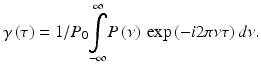
(6.12)
The importance of this Fourier relation cannot be overemphasized. It is the basic theorem that links time domain with frequency domain interferometry. The superposition of the individual backscattered fields together with the reference wave will form interference fringes only if the temporal delays between the different light fields are smaller than the range of temporal coherence. According to the bandwidth product, the width of the coherence function must be inversely proportional to the spectral bandwidth of the light source. For Gaussian-shaped power spectral density, the expression for the coherence length becomes
(6.13)
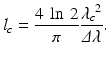
The axial resolution of any OCT system is given by half the coherence length since the wave travels twice the sample arm. The temporal coherence function is equal to the normalized field autocorrelation function Γ(τ) = 〈E(t), E(t − τ)〉, with brackets indicating an ensemble average. In the case of statistically stationary fields, the ensemble average equals time average. The complex degree of coherence is then defined as the normalized temporal coherence function γ(τ) = Γ(τ)/Γ(0). If we use now our definition of the structure function g(z), we finally obtain from Eq. 6.11 the expression for the absolute value of the measured Fourier domain signal:
![$$ \begin{array}{c}\left|{I}_D\left(\tau \right)\right|\propto {I}_0\left|\gamma \left(\tau \right)\right|\left[{\displaystyle \sum_i}{\left|{\rho}_i\right|}^2+{\left|{\rho}_R\right|}^2\right]\\ {}+{I}_0\left|\gamma \left(\tau \right)\right|\otimes \left[{\displaystyle \sum_{i,j;i>j}}{\rho}_i{\rho_j}^{*}\delta \left[\tau -\left({\tau}_i-{\tau}_j\right)\right]+{\displaystyle \sum_i}{\rho}_i{\rho_R}^{*}\delta \left[\tau -\left({\tau}_i-{\tau}_R\right)\right]\right]+c.c.\end{array} $$
” src=”/wp-content/uploads/2017/03/A76297_2_En_7_Chapter_Equ14.gif”></DIV></DIV><br />
<DIV class=EquationNumber>(6.14)</DIV></DIV>where <SPAN class=EmphasisTypeItalic>τ</SPAN> = <SPAN class=EmphasisTypeItalic>z</SPAN>/<SPAN class=EmphasisTypeItalic>c</SPAN> and δ(<SPAN class=EmphasisTypeItalic>τ</SPAN>) is the Dirac delta function. The first term of the rhs corresponds to the total intensity of the signal that appears as DC term at <SPAN class=EmphasisTypeItalic>τ</SPAN> = 0. The following two terms are self-cross correlations between fields back-reflected at individual sample structure layers. These terms are commonly referred to as autocorrelation terms or coherence noise terms. Only the last two terms actually display the actual axial sample structure. Still there is an ambiguity with respect to the zero delay associated with the Hermitian nature of the inverse Fourier transform as it is applied to the real-valued signal <SPAN class=EmphasisTypeItalic>I</SPAN> <SUB><SPAN class=EmphasisTypeItalic>D</SPAN> </SUB>. Each structure term has its mirror term in the adjoint Fourier space. Figure <SPAN class=InternalRef><A href=]() 6.2 shows the signal measured by FdOCT instrument and how this signal is processed to obtain the reconstruction corresponding to amplitudes of back-reflected intensity versus one-dimensional distribution of scattering points (optical A-scan).
6.2 shows the signal measured by FdOCT instrument and how this signal is processed to obtain the reconstruction corresponding to amplitudes of back-reflected intensity versus one-dimensional distribution of scattering points (optical A-scan).
Get Clinical Tree app for offline access

Fig. 6.2
Reconstruction of the axial structure of an object in FdOCT: structural information, DC signal, and coherence noise terms are residual in the amplitude spectrum of the spectral fringe signal
All three extra signal components described by Eq. 6.14 (DC signals, coherence noise, and symmetrical redundant image) limit the useful measurement range and can lead to misinterpretation of reconstructed structure. There are two main types of the coherence noise in FdOCT. The first type represented by term is associated with mutual interferences of light waves back-reflected or scattered from different points within a measured object, located along the penetration beam. In this case each light wave can interfere with others and gives contribution to OCT signal. This signal is present in OCT images even if the reference arm of the interferometer is blocked. Another source of coherence noise affecting Fourier domain imaging is caused by interference of light waves scattered from optical components of the OCT system. Due to the high sensitivity of FdOCT imaging and relatively long axial coherence range (some millimeters), the contribution of light scattered on optical components of the OCT device can be significant. In order to avoid an overlap between various signal components, one needs to take care that all structure terms are confined to one half space.
In practice one adjusts the reference arm delay accordingly. Figure 6.3 shows results of image reconstruction for a sample consisting of four reflecting interfaces. Three measurements have been simulated with different positions of the reference mirror. In the first case (Fig. 6.3a), the optical distance (optical path delay) between reference mirror and the sample is longer than the thickness of the entire set of four interfaces. This enables distinguishing between sample and coherence noise artifacts. Shortening the distance between the reference mirror and the sample can lead to overlapping of terms representing the sample and the coherence noise. In result the structure cannot be distinguished (Fig. 6.3b). The situation can be even more complex when the virtual position of the reference mirror is placed “inside” the object. In this case both the coherence noise terms and symmetrical images mix altogether with the signal representing the actual axial sample structure. In both cases (Fig. 6.3b, c), direct reconstruction of true architecture of the measured sample is impossible.
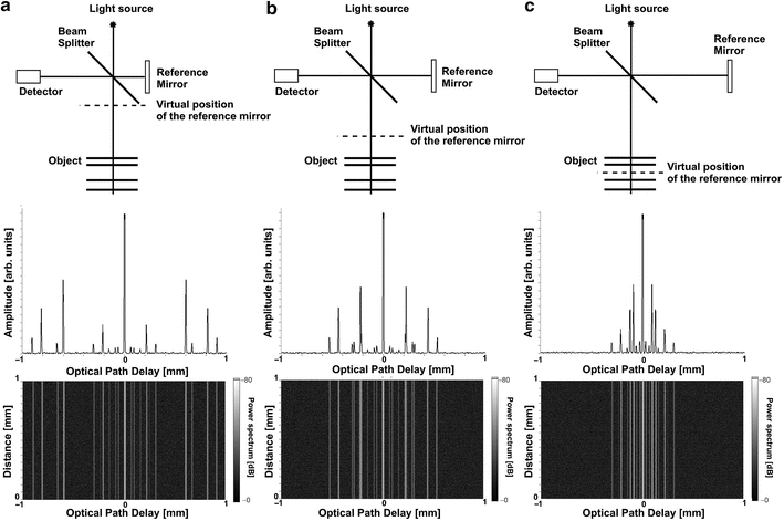
Fig. 6.3
Simulation of Fourier domain OCT reconstruction for a sample comprising four smooth reflecting interfaces registered for three different positions of the reference mirror. Upper row shows the scheme of the interferometer configuration chosen for each measurement. Middle and bottom rows demonstrate axial scans and cross-sectional images, respectively
Usually the coherence noise components introduced by the object structure are irregular and distributed close to the zero optical path delay. In contrary coherence noise terms associated with light reflections from optical components of the device usually create characteristic regular stripe patterns, which are randomly distributed along the axial direction (Fig. 6.4). To eliminate such coherence noise terms, it is sufficient to register the spectral fringe pattern in the absence of the sample (background) and subtract it from the spectral fringes registered with the sample in place. Assuming that mutual interferences between light waves scattered from optical components of the OCT system and sample interfaces are negligible, the simple subtraction procedure can effectively reduce the regular stripe pattern that otherwise disturbs the reconstructed cross-sectional image. Practically it is possible to measure the background signal by deflecting the sample beam in an OCT interferometer during the background measurement. Random instabilities of the optical system, which are usually present in OCT devices, such as mechanical vibrations of optical components or thermal expansion of optical fibers can be taken into account and compensated by using an average over several spectral fringe patterns of the background signal. Figure 6.4b shows an example of the background subtraction algorithm applied to a FdOCT tomogram of the human retina measured in vivo.
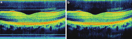
Fig. 6.4
Cross-sectional images of the human retina in vivo (macular region) obtained by FdOCT: (a) including all coherence noise terms, (b) after background subtraction
Nevertheless the autocorrelation terms will still be present (Fig. 6.4) and give rise to coherent noise background that may lead to misinterpretation of the actual sample structure. The question arises whether it is possible to remove all coherence noise terms together with the inherent ambiguity of the FdOCT signal. An answer can be found by taking advantage of the fact that FdOCT being an interferometric method is sensitive to the relative phase between the individual fields that coherently add up at the detector. Note that in particular any reference delay τ R will only affect the phase of the structure terms in Eq. 6.14 but has no effect on the autocorrelation and the DC terms. This observation is the basis for phase-shifting techniques that eventually allow for the elimination of all signals apart from the true structure terms. The important fact is that these methods allow a direct reconstruction of the true depth resolved phase function of the sample field and thus of the complex valued structure function g(z) Eq. 6.3.
In practice it is often impossible to predict the thickness of measured sample. Artifacts created by coherence noise terms may be misinterpreted as details of a real structure. This problem arises, paradoxically, as a result of the high sensitivity of FdOCT. The FdOCT imaging is performed at an optical energy (optical power multiplied by exposure time) that is about hundredfold lower than for traditional time domain OCT. It is therefore tempting to increase optical power to the same energy level in order to enhance sensitivity. Unfortunately, beneficial results of higher power on the sensitivity level are counterbalanced by the fact that simultaneously artifacts caused by coherence noise will emerge and will be visible above shot noise. However, it is possible to choose optimal optical power levels used for FdOCT imaging to keep the coherence noise components under the shot noise level [50]. Illustration of this phenomena is presented in Fig. 6.5. Coherence noise artifacts can be observed, for example, in retinal imaging as a result of cross-interference of waves originating from two strongly reflecting layers in the retina: internal limiting membrane (ILM) and retinal pigment epithelium (RPE). Figure 6.5 demonstrates an influence of the total exposure time (sensitivity) on the visibility of the coherence noise artifacts in retinal FdOCT imaging. Using 740 μW of optical power of light entering the eye and 256 μs of exposure time, several parasitic cross correlations produce artificial features, which are especially visible above the right part of the retinal surface in Fig. 6.5a. It is easy to verify that distances between ILM and structures around RPE match distances between position τ = 0 and corresponding artifacts. The eightfold reduction of the exposure time (−9 dB in sensitivity) results in strong suppression of those artifacts (Fig. 6.5b). Under these circumstances the quality of the image is sufficient to delineate all retinal layers.
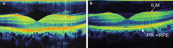
Fig. 6.5
Spectral OCT cross-sectional images of the retina in vivo (macular region). The images were taken with (a) 256 μs/A-scan (103 dB sensitivity) and (b) 32 μs/A-scan (94 dB sensitivity). Coherence noise components are clearly visible in the top of the panel (a), while for (b) the dominant noise is the shot noise; ILM inner limiting membrane, PR photo receptors, RPE retinal pigment epithelium. Arrows in (a) indicate the equal optical distances
Considering the measurement configuration with significant contribution of the coherence noise terms, their amplitudes may be expressed as
where ρ = e − η/hv is the efficiency of photoelectric conversion of photodetector, e − is an electron charge, η is the total efficiency of the spectrometer, h is Planck’s constant, P 0 is the integrated optical power of the beam entering the interferometer assumed to be Gaussian across optical frequencies  double path coupling ratio of the beam splitter, N is the number of samples taken in optical frequency domain, and R m,n are reflectivities of consecutive back-reflecting or scattering points in the object distributed along the probing beam.
(6.15)
double path coupling ratio of the beam splitter, N is the number of samples taken in optical frequency domain, and R m,n are reflectivities of consecutive back-reflecting or scattering points in the object distributed along the probing beam.The most optimal performance of OCT instruments is usually achieved with shot noise as the dominant source of noise. In FdOCT the signal registered by the detector is Fourier transformed. Therefore, the power spectrum of the resultant shot noise may be expressed as [50]
where T is the exposure time needed to register one A-scan (N samples in Fourier domain), R ref is the effective reflectivity of the reference mirror, and R n is the reflectivity of consecutive back-reflecting or scattering point in the sample distributed along the probing beam. The ratio of coherence noise to shot noise in terms of electrical power of obtained signals is expressed by
(6.16)
(6.17)
In order to simplify Eq. 6.17, let us assume that there are only two strongly reflecting interfaces with identical reflectivity R contributing to the coherence noise. In this case the ratio of the coherence noise terms to the shot noise may be expressed as
(6.18)
Plots of the ratio of coherence noise to shot noise level as a function of sample reflectivity calculated according to Eq. 6.18 are shown in Fig. 6.6. These theoretical plots are calculated for two values of dynamic range corresponding to detection using spectrometer (DR = 72 dB) and swept source system with photodiode in dual balanced configuration (DR = 85 dB). For these calculations the value of input optical power was assumed to be P0 = 2 mW (740 uW reaching the object), the double path coupling ratio κ = 0.20, and the spectrometer efficiency η = 0.14 and the double path losses associated with collimating, back coupling to the fiber, passing through X–Y scanner to be 0.4. These parameters give sensitivities from 82 to 106 dB for exposure times varying from 2 to 512 μs per A-scan measured close to the zero path delay.
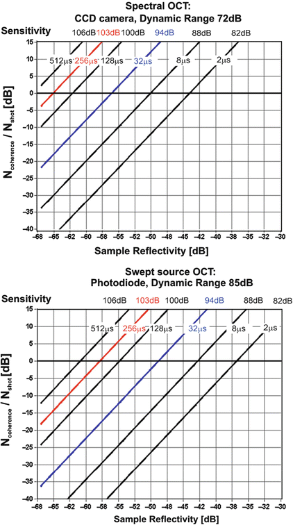
Fig. 6.6
Ratio of coherent noise to shot noise versus reflectivity of the sample calculated from (Eq. 6.17) for different values of exposure time, corresponding sensitivity, and dynamic range. The optimal exposure time to perform an experiment avoiding coherence noise terms from two surfaces of reflectivity R can be chosen by taking exposure time values, for which the oblique lines presented in the graphs are localized below 0 dB horizontal line. Red and blue lines were calculated for exposure times used in the retinal experiment, which results are shown in Fig. 6.5
The analyzed range of reflectivity values (i.e., −30 dB to −70 dB) and sensitivities (82–106 dB) covers the typical values of reflectivity and sensitivity used in biomedical imaging. For example, in retinal OCT imaging the most reflective layers in the posterior eye are inner limiting membrane (ILM) and retinal pigment epithelium (RPE). Coming back to results presented in Fig. 6.5, the imaging parameters of FdOCT system are given above and were also used to plot relations presented in Fig. 6.6. Cross-sectional retinal images were obtained twice in the same subject using two values of exposure time: 32 us and 256 us. Taking into account the exact value of the instrument sensitivity, it was possible to find the effective average reflectivities of ILM in the presented OCT scans to be approximately −60 dB. Using the graph shown in Fig. 6.6 along with measured values of effective reflectivity of retinal layers, it is possible to estimate the maximum sensitivity corresponding to coherence noise-free imaging of the posterior segment of the human eye to be approximately 97 dB in spectral OCT systems (72 dB of dynamic range) and 102 dB (85 dB of dynamic range) in swept source OCT. The abovementioned optimization causes a limitation of the sensitivity and dynamic range. For example, in the system characterized by the dynamic range of originally 85 dB, it is possible only to image without coherence noise artifacts within a dynamic range of 45 dB.
The limitation of dynamic range due to power optimization can be overcome by using a dual balanced detection (called also differential Fourier domain detection method (dFdOCT)) [6, 51]. This method takes advantage of the fact that terms carrying direct information on the location of reflecting layers depend on the reference mirror position, while the remaining coherence noise terms do not (see Eq. 6.14). In order to completely remove the parasitic terms, it is sufficient to measure one additional spectral fringe pattern I D (k), with a phase shift of π introduced into the reference arm. Subtraction of these two spectral fringe patterns will yield terms associated exclusively with the sample structure. The π phase shift of the reference beam in differential measurements can be achieved either mechanically by attaching the reference mirror to a moving element such as a piezo actuator or electro-optically, e.g., by a phase modulator placed in the reference arm of the interferometer. The effective measurement time is doubled as compared to standard FdOCT. In swept source OCT it can be also realized by using differential measurement with additional fiber coupler introducing adequate phase shift for two detection channels (the so-called dual balanced detection). Figure 6.9a, b show examples of cross-sectional images of porcine anterior segment obtained with standard and the differential FdOCT technique. The coherence noise and strong DC signal in the central part of the image representing zero path delay are totally removed after two-frame procedure. Nevertheless, the overlap between conjugate images is still present and can only be removed by application of complex FdOCT techniques.
6.3 Complex Fourier Domain Optical Coherence Tomography
The Fourier transform of the real-valued spectrum yields redundant information for positive and negative fringe frequencies corresponding to positive and negative path length differences between the sample and the reference. Even using the coherence noise-free imaging, one needs to adjust the reference arm delay so that it is slightly shorter than the relative distance of the first sample interface. In this case the axial structure does not mix with its mirrored representation in the conjugate Fourier half space. Hence only half of the Fourier space can be used for the sample structure.
The reconstruction of the complex representation of spectral fringe signal resolves this ambiguity and the image space is doubled (Fig. 6.9c). This needs at least two phase-shifted copies (the so-called frames) of the cross correlation between sample and reference signal. The most straightforward realization of the phase shift is done by changing the path length of the reference arm using, for example, a mirror mounted on a moving mechanical element (Fig. 6.7). A faster and more precise way of shifting the optical delay in the reference arm using electro-optic modulator has been reported by Gotzinger et al. [37]. An alternative approach has been used by Yasuno et al. where phase-shifted spectra are recorded simultaneously on different lines of an area detector [38]. However, the need for an area detector reduces the speed performance of the technique and the light efficiency is critical.
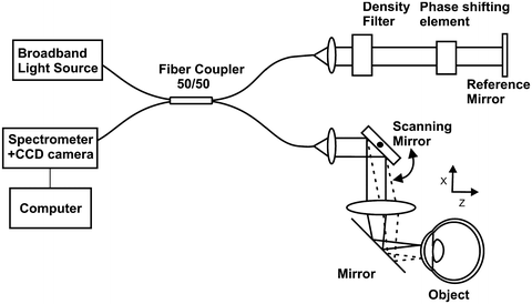
Fig. 6.7
Drawing of spectral OCT system with phase-shifting element used for complex OCT measurements. Similar to other SOCT devices, the system is based on the Michelson interferometer setup with custom-designed highly efficient spectrometer with high-speed linear photodetector. The sample arm enables lateral scanning of probing light beam. The difference between complex SOCT instrument and standard spectral OCT system is in additional phase-shifting device placed in the reference arm and more complex electronic synchronization of the lateral scanners, the phase shifter, and the spectrometer
6.3.1 Complex Two-Frame Technique
In principle the complex reconstruction can be based only on two frames with a relative phase shift of π/2 [29]:
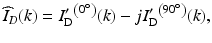
where the role of the dashes will be explained in due course. A simple combination of two shifted spectra will still suffer from a strong DC component as well as coherence noise terms. The necessary approximation is that the reference intensity is much larger than the sample intensity which is the case in most biomedical applications. Then it is sufficient to subtract a reference spectrum from each spectral interference pattern and one is effectively left with a small sample intensity DC term together with the cross-correlation terms.
(6.19)
In this case the dashes in Eq. 6.19 indicate that a reference subtraction has been applied. Since only two phase-shifted copies of the recorded interference pattern are needed, it is possible to realize fast complex in vivo spectral FdOCT systems [37]. However, as pointed out such method works only well for a limited range of optical bandwidths.
For wavelength tuning FdOCT on the other hand, it is possible to perform true heterodyne detection by locking the detector to a sinusoidal reference arm delay modulation. In this case the dashes indicate that only the modulated cross-correlation terms between reference and sample are considered.
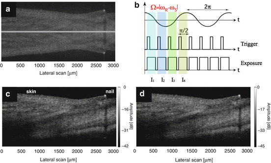
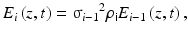
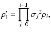
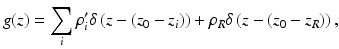
One way to achieve a wavelength-independent modulation of the actual structure terms in Eq. 6.14 is to employ frequency-shifting devices such as acousto-optic frequency shifters (AOFS). They are easy to implement into FdOCT systems based on wavelength tuning and allow for high-speed quadrature detection with fast PIN diodes [33, 34]. Nevertheless for spectral FDOCT systems, the array detectors cannot follow the fast signal modulations in the MHz range. Bachmann et al. demonstrated a solution using two slightly detuned AOFS in the sample and reference arm respectively [52]. A quadrature detection scheme is realized by locking the array detector to the resulting lower beating frequency and recording the shifted spectral interference patterns via an integrated bucket method as shown in Fig. 6.8b. Figure 6.8a shows a tomogram of the fingernail region evaluated with standard FdOCT. The strong overlapping between sample structure and its mirror adjoint renders it impossible to determine the actual structure. Figure 6.8d demonstrates the capability of complex signal reconstruction based on Eq. 6.19. A reference subtraction has been performed; nevertheless a spurious DC term might still be visible. Figure 6.8c shows the result if a complex differential technique is applied. Such reconstruction is achieved by the substitution I′ D (0°) = I 1 − I 3 and I′ D (90°) = I 2 − I 4 (Fig. 6.8b) into Eq. 6.2 [52]. It should however be mentioned that integrated bucked methods used in spectral OCT suffer in general from fringe washout, an effect discussed in Sect. 6.3.6. Still, this method has the potential together with array detectors based on CMOS technology to perform true heterodyne detection with spectral OCT. CMOS technology allows on-chip demodulation of the heterodyne signal such that only the AC part will subsequently be amplified and digitized.