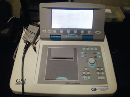
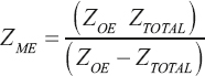
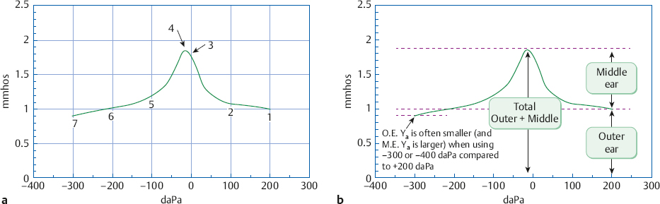
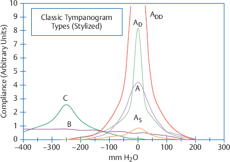
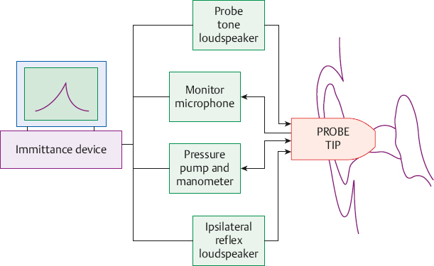
7 Acoustic Immittance Assessment We learned in Chapter 1 that acoustic immittance is the general term used to describe the various aspects of acoustic impedance and admittance. Let us quickly review the major terms. Acoustic impedance (Za) is the opposition to the flow of sound energy, measured in ohms. Acoustic impedance is the ratio of sound pressure (P) to sound flow, or volume velocity (U); or Za = P/U The reciprocal of acoustic impedance is acoustic admittance (Ya), expressed in acoustic millimhos (mmhos). Acoustic admittance is the ease of sound flow, or Ya = U/P Acoustic impedance is composed of (1) a frictional component called acoustic resistance (Ra), (2) a stiffness component called negative (stiffness) acoustic reactance (–Xa), and (3) a mass component called positive (mass) acoustic reactance (+Xa). Their reciprocals are respectively the components of acoustic admittance: (1) acoustic conductance (Ga), (2) positive (compliant or stiffness) acoustic susceptance (+Ba), and (3) negative (mass) acoustic susceptance (–Ba). The immittance of the ear is derived from its various sources of mechanical and acoustical springiness, mass, and resistance (Van Camp, Margolis, Wilson, Creten, & Shanks 1986): (1) The stiffness (springiness) components come from the volumes of air in the outer ear and middle ear spaces, the tympanic membrane, and the tendons and ligaments of the ossicles. (2) The mass components are due to the ossicles, the pars flaccida of the eardrum, and the perilymph. (3) Resistance (friction) is introduced by the perilymph, the mucous membrane linings of the middle ear spaces, the narrow passages between the middle ear and mastoid air cavities, and also by the tympanic membrane and the various middle ear tendons and ligaments. Contractions of the middle ear muscles also change the immittance of the ear, usually by increasing the stiffness component. Various pathologies cause changes in the admittance characteristics of the ear that can help us to detect their presence and to distinguish among them. This is why we use acoustic immittance testing in clinical audiology. Admittance measurements are employed clinically because they are more straightforward than those using impedance. The acoustic admittance characteristics of the ear can be assessed using a device such as the one described in Fig. 7.1. The acoustic immittance of the ear is measured by inserting an ear piece called a probe tip into the ear canal. The probe tip is encased in a flexible plastic cuff to create an airtight connection between the ear canal and the probe tip, called a hermetic seal. The probe tip includes four tubes. One tube is connected to a receiver (loudspeaker), which is used to deliver a tone into the ear canal. This sound is called the probe tone. The second tube is connected to a measuring microphone and is used to monitor the probe sound within the ear canal. The third tube is connected to an air pressure pump and manometer (pressure meter), and the fourth tube connects to another receiver used to present stimuli for testing the acoustic reflex. In addition to the probe tip in one ear, a second earphone goes to the opposite ear and is used for acoustic reflex tests. The latter earphone may be a standard audiometric earphone or an insert receiver, depending on the device being used. The acoustic admittance (in mmhos or ml) measured with such a device is displayed on a video screen or meter and is usually plotted on paper. Fig. 7.2 shows a photograph of a typical clinical acoustic immittance instrument. The process of measuring the ear’s admittance employs the first two tubes just described, i.e., those connected to the receiver that produces the probe tone, and to the measuring microphone. The basic approach is to introduce an 85 dB sound pressure level (SPL) probe tone into the ear canal, where it will be affected by the admittance properties of the ear. This will be revealed as an increase or decrease in the level of the probe tone as it is monitored by the measuring microphone. The details of immittance device technology are beyond the scope of this book, but the beginning student should be aware that instruments called bridges involve a manual intensity adjustment to bring the probe level in the ear to 85 dB SPL, whereas those referred to as meters use an automatic volume control to keep the probe level at 85 dB SPL. In addition to measuring overall admittance (Y), most admittance meters also provide separate measurements of susceptance (B) and conductance (G). This is done by analyzing the monitored signal in terms of in-phase (for G) and out-of-phase (for B) components. The characteristics and calibration of acoustic immittance devices are given in the ANSI S3.39 (2012) standard. Most routine immittance tests use a 226 Hz (or a 220 Hz) probe tone. Low-frequency probe tones such as these were originally chosen because they are sensitive to changes in stiffness reactance, comprising a major part of the normal ear’s impedance. In addition, admittance devices are calibrated in terms of the admittance of an equivalent volume of air. In other words, when the meter indicates that the admittance of an ear is 1.8 mmhos at 226 Hz, it means that the admittance of the ear corresponds to that of a 1.8 ml (ml) volume of air. Let us see why. Suppose we have several stainless steel containers (i.e., hard-walled cavities) with various volumes, ranging from perhaps 0.2 to 2.5 ml. The air volume in such a cavity constitutes an acoustical spring, so that its admittance is essentially a compliant susceptance (and its impedance a stiffness reactance). Inserting our probe tip into each of these containers would show that admittance increases (or the impedance decreases) as the volume of the cavity becomes larger. Repeating this experiment with different probe tone frequencies in the same cavity would result in different amounts of admittance at each frequency. This reflects the fact that admittance depends on frequency. We would also find that admittance (in mmhos) is equal to the volume (in ml when the probe tone is 226 Hz). For example, the acoustic admittance (Ya) at 226 Hz will be 2.0 mmhos for a 2 ml container, 1.2 mmhos for a 1.2 ml container, 0.3 mmho for a 0.3 ml volume, etc. This is why 226 Hz has become the preferred low-frequency probe tone frequency. Higher-frequency probe tones provide other kinds of information and are often used as well. Fig. 7.2 An example of a clinical acoustic immittance device. For diagnostic purposes we are mainly concerned with the immittance of the middle ear because it provides information about (1) middle ear pathologies and (2) middle ear muscle contractions due to the acoustic reflex. However, the probe tip monitors the immittance of the ear from the perspective of its location, which is in the general vicinity of the ear canal entrance. Thus, the probe tip measures the total immittance of the ear, which includes the combined effects of the outer ear and the middle ear. This is a problem because ear canal volume (size) is usually not clinically relevant, yet its influence on the total immittance value (at the probe tip) is often big enough to cloud the effects of the clinically significant middle ear immittance value. For example, a patient with abnormally low middle ear admittance due to a conductive disorder may have a normal total admittance value due to a large ear canal volume. Another individual whose middle ear is normal might seem to have unusually low total admittance because her ear canal volume is quite small. A third patient might have low total admittance due to otitis media when first evaluated. The middle ear problem might be completely resolved (i.e., the middle ear immittance has returned to normal) when she returns for reassessment, but the total Ya might still be abnormally low simply because her outer ear volume was made to appear smaller by a very deeply inserted probe tip. This can happen because the volume under the probe tip will be different depending on how deeply it has been inserted. We must remove the outer ear component from the total admittance value at the probe tip to get an undistorted representation of the middle ear’s admittance at the eardrum. In other words, removing the effect of the ear canal moves the measurement location from the end of the probe tip to the plane of the tympanic membrane. We can achieve this goal by taking advantage of the fact that total admittance (YTOTAL) is simply the sum of the admittances of the outer ear (YOE) and the middle ear (YME)1: YTOTAL = YOE + YME Consequently, subtracting the admittance of the outer ear from the total admittance leaves the middle ear admittance, which is the value that we need: YME = YTOTAL − YOE This simple, additive relationship is one of the main reasons why we use measurements based on admittance rather than impedance.2 The procedure for determining the admittance of the middle ear (i.e., at the plane of the ear drum) is simple and straightforward: The first step is to measure the total admittance (YTOTAL) of the ear (Fig. 7.3a). The second step is to measure the ear’s admittance again while pressure is being exerted on the tympanic membrane. This measurement reflects the admittance of the outer ear (or ear canal) alone, and is depicted in Fig. 7.3b. The pressure change is accomplished using the pressure pump connected to one of the tubes in the probe tip. The rationale for this tactic is that the heightened air pressure puts the eardrum under so much tension that it acts like a hard wall, so that essentially no sound energy can be transmitted into the middle ear. This strategy prevents the probe tip from measuring the admittance of the middle ear. In this case, we say that the middle ear has been excluded from the measurement. Hence, the admittance obtained under these conditions comes from the outer ear alone. We now know the total admittance (of the outer and middle ear combined) from the first measurement and the admittance of the outer ear from the second measurement. The third step (Fig. 7.3c) is to figure out the previously unknown middle ear admittance (YME) by simply subtracting the outer ear admittance (YOE) from the total admittance (YTOTAL). Tympanometry involves measuring the acoustic admittance of the ear with various amounts of air pressure in the ear canal. We can control the amount of air pressure in the ear canal because the probe tip makes an hermetic seal with the ear canal, and one of its tubes is connected to an air pump and manometer. The amount of air pressure is expressed in terms of dekapascals (daPa) or of millimeters of water pressure (mm H2O),3 relative to the atmospheric pressure in the room where the test is being done. Hence, 0 daPa implies that the pressure in the ear canal is equal to the atmospheric pressure, positive pressure (e.g., +100 daPa) means that the ear canal pressure is greater than atmospheric pressure, and negative pressure (e.g., –100 daPa) means it is less than atmospheric pressure. This information is shown on a diagram called a tympanogram (Fig. 7.4a), with admittance in mmhos or (or equivalent volume in ml) on the y-axis, and pressure in daPa (or mm H2O) on the x-axis. Notice in the figure that atmospheric pressure (0 daPa) is in the middle, with positive pressure increasing to the right and negative pressure increasing to the left. 1 YME can also called YTM, which stands for the admittance at the plane of the tympanic membrane. 2 The equivalent impedance formula is more complicated: where ZTOTAL is the total impedance, ZOE is outer ear impedance, and ZME is middle ear impedance. Fig. 7.3 (a) Total admittance (YTOTAL) at the probe tip includes the combined admittances of the outer and middle ear. (b) The middle ear is excluded from the admittance measurement by using air pressure to tense the eardrum. The probe tip now registers the admittance of just the outer ear (YOE). (c) Admittance at the plane of the drum, or middle ear admittance (YME), is inferred by subtracting YOE from YTOTAL. Because most instruments generate tympanograms automatically, we can concentrate on what is happening and why. (Here, as elsewhere, it is assumed that the ear and related structures have already been inspected.) The first step in tympanometry is to properly insert the probe so that it makes a hermetic seal with the external auditory meatus. The probe tip should face the drum and not the ear canal wall, and the path to the tympanic membrane should not be blocked. Cerumen will be problematic if it gets into the probe tip tubes or completely obstructs the path to the tympanic membrane, but the simple presence of some wax is usually not a problem. The next step is to select the probe frequency and the admittance parameter(s) to be measured. We will measure overall acoustic admittance (Y) with a 226 Hz probe tone. The appropriate button(s) on the immittance device are then pushed to initiate the following tympanometry procedure. The 226 Hz probe tone is turned on and the pressure in the ear canal is then raised to +200 daPa. This amount of positive pressure is usually assumed to tense the eardrum sufficiently to prevent the admittance of the middle ear from being measured, as described in the previous section and illustrated in Fig. 7.3b. A useful analogy is to imagine that the +200 daPa pressure causes the tympanic membrane to become “opaque” to sound, so that the probe cannot “see” the middle ear through it. Thus, the admittance obtained at +200 daPa is assumed to represent just the outer ear. In Fig. 7.4a, the admittance at +200 daPa is 1.0 mmho (point 1). This means that the acoustic admittance of the outer ear is 1.0 mmho, and that the ear canal volume is 1.0 ml because mmhos equals volume at 226 Hz. The air pressure is then decreased at a steady rate while we continue to measure the admittance. Notice that the tympanogram curve slowly rises as the pressure decreases below +200 daPa. The total admittance rises by ~ 0.1 mmho, to reach 1.1 mmhos, when the pressure is +100 daPa (point 2). It then increases more rapidly as the pressure drops further, and achieves 1.75 mmhos at 0 daPa, or at atmospheric pressure (point 3). Why is this happening and what does it mean? As the pressure in the ear canal is steadily reduced, the tension on the tympanic membrane also diminishes. The middle ear is no longer being completely blocked from the view of the probe tip. Instead, the probe tip is now picking up more and more of the middle ear’s admittance. The less the pressure, the less the tension on the eardrum, and the more the middle ear contributes. It is as though the eardrum has changed from being completely “opaque” to being progressively more “translucent.” Because we know that 1.0 mmho is coming from the ear canal, we can deduce that the additional amounts of admittance (above 1.0 mmho) must be coming from the middle ear. Hence, the 1.75 mmhos of total admittance at 0 daPa represents 1.0 mmho from the ear canal and 0.75 mmho from the middle ear. Fig. 7.4 (a) Example of an admittance (Y) tympanogram obtained at 226 Hz (or 220 Hz). Numbers refer to the text. (b) The same 226 Hz admittance tympanogram labeled to show total acoustic admittance, outer ear acoustic admittance, and middle ear (or peak-compensated static) acoustic admittance. Returning to the tympanometry procedure, the pressure continues to be reduced below 0 daPa. Air is now being pumped out of the ear canal instead of into it, so that the pressure is becoming increasingly negative. We see that the admittance continues rising until it reaches a maximum of 1.85 mmhos when the pressure in the outer ear is –15 daPa (point 4). The total admittance then begins to fall again as the negative pressure increases. The maximum point is called the peak of the tympanogram. Using our visual analogy, this is where there is no longer any tension being imposed on the tympanic membrane, so that it becomes “transparent,” allowing the probe tip to “see” all of the middle ear admittance. Because we know that the maximum (or peak) total admittance is 1.85 mmhos and that the outer ear admittance is 1.0 mmho, we can deduce that the middle ear admittance is 0.85 mmho. (The middle ear admittance is often referred to as the static admittance, or more accurately as peak-compensated static admittance, discussed below.) By reducing the pressure below 0 daPa we are actually increasing the negative pressure. This causes the admittance to fall to 1.2 mmhos at –100 daPa (point 5), and to 1.0 mmho at –200 daPa (point 6). The falling admittance values indicate that the negative pressure is tensing the tympanic membrane, so that it again becomes progressively more opaque to sound. Continuing to increase the negative pressure causes the admittance to fall to only 0.9 mmho at –300 daPa (point 7), which is the lowest pressure used here. Thus, the admittance at –300 daPa is actually smaller than it was at +200 daPa. This means that the middle ear can be excluded from the measurement by applying either positive or negative pressure (i.e., at point 1 or 7; these two points are often called the positive and negative “tails”). Even though many audiologists use +200 daPa to estimate outer ear volume, the lowest point on the tympanogram is often obtained at –300 to –400 daPa. Compared with +200 daPa, it has been shown that –400 daPa more effectively removes the middle ear admittance and thus provides a more accurate measure of the outer ear volume (Shanks & Lilly 1981). It is suggested that (1) tympanograms should be obtained over a pressure range from +200 daPa down to –400 daPa (or at least –300 daPa); and that (2) the admittance of the middle ear should be based on (a) the tympanogram peak as the total admittance value and (b) the lower of the two “tails” as the outer ear admittance value. Fig. 7.4a is redrawn in Fig. 7.4b to summarize the major components of the typical 226 Hz (or 220 Hz) tympanogram. Because the y-axis shows admittance in mmhos (or equivalent volume in ml), the overall height of the peak relative to 0 mmhos gives total admittance, and the overall height of the “tail” (at +200 daPa or –300 daPa) gives the outer ear volume. The height of the tympanogram’s peak above its own baseline (i.e., one of the two tails) gives the middle ear admittance. The peak of the tympanogram also provides us with an estimate of the pressure within the middle ear, which is –15 daPa in this example. Here is why: Recall that we exclude the middle ear by using air pressure to stress the eardrum. This stress occurs because there is more pressure on one side of the tympanic membrane than on the other (higher pressure in the outer ear than in the middle ear, or vice versa). The admittance will be highest (the peak) when the eardrum is not experiencing any stress due to a pressure difference. Thus, the positive or negative pressure used to obtain the peak pressure should be the same as the pressure that exists on the other side of the eardrum, that is, within the middle ear. This is so because having the same pressure on both sides of the eardrum will result in the least tension on the drum, and hence the highest total admittance value, so that the tympanogram peak provides us with an estimate of the pressure inside the middle ear. The major considerations that come into play when interpreting 226 Hz (or 220 Hz) tympanograms include static acoustic admittance, tympanometric gradient or width, ear volume, the pressure at which the tympanometric peak occurs, and the shape of the tympanogram. It is also possible to categorize tympanograms into a reasonably small number of types that summarize the majority of configurations found clinically. Several systems have been proposed for classifying 220 Hz (226 Hz) tympanograms (Lidén 1969; Jerger 1970; Lidén, Peterson, & Björkman 1970; Jerger, Anthony, Jerger, & Mauldin 1974; Lidén, Harford, & Hallén 1974; Feldman 1975; Paradise, Smith, & Bluestone 1976; Silman & Silverman 1991). The most widely utilized tympanogram classification system was originated by Jerger (1970). Fig. 7.5 shows most of the tympanogram types in this system. These types were based on relative tympanograms obtained with an immittance bridge, and this format is retained in the figure. Notice that these tympanograms are expressed in arbitrary compliance units instead of absolute admittance in mmhos (static acoustic admittance and ear canal volume were measured separately). Type A tympanograms had a distinctive peak in the vicinity of atmospheric pressure and were typical of normal patients, as well as those with otosclerosis. If the type A tympanogram had a very shallow peak, it was classified as type AS, which was generally associated with otosclerosis but could also occur with otitis media. In contrast, very high (deep) type A tympanograms were designated as type AD. These were found in otherwise normal ears that had scarred or flaccid eardrums, or in cases of ossicular interruptions. The type ADD tympanogram was so deep that the peak was off-scale, and was found in ears with ossicular discontinuities. Type B tympanograms were essentially flat across the pressure range, and were characteristic of patients with middle ear fluid and cholesteatoma. However, type B tympanograms can also be caused by entities such as eardrum perforations or impacted cerumen (or other obstructions) in the ear canal. Type C tympanograms had negative pressure peaks beyond –100 daPa (mm H2O), indicating negative middle ear pressure. They were associated with Eustachian tube disorders, and were also found in cases of middle ear fluid. Not shown in the figure are tympanograms with notched peaks, which were classified as type D if the notch was narrow and type E if it was wide. These are rare occurrences when using 226 Hz (220 Hz) probe tones. Type D was associated with hypermobile or scarred (but otherwise normal) eardrums, whereas type E was found in cases of ossicular disruption. Static acoustic immittance is the immittance of the middle ear at some “representative” air pressure. It was originally considered to be the middle ear impedance or admittance obtained under conditions of atmospheric pressure (Zwislocki & Feldman 1970; Feldman 1975, 1976). This point might seem confusing because we pressurized the ear to figure out the middle ear admittance. However, remember that the total admittance can be measured without applying any pressure, that is, at atmospheric pressure of 0 daPa. Pressure is used to stiffen the eardrum to obtain the outer ear component. This “pressurized” outer ear value is then removed from the total admittance at atmospheric pressure, leaving the middle ear admittance at the eardrum, which is also at atmospheric pressure. In any case, this is the situation that presumably exists in the patient’s ear “under regular conditions” when the probe tip is not there. On the tympanogram, it is the value of YME obtained at 0 daPa, which is 0.75 mmho in Fig. 7.4a (point 3). We will call this measurement “atmospheric static.” The alternative approach is to measure static admittance at whatever pressure corresponds to the peak of the tympanogram (Brooks 1969; Jerger 1970; Jerger, Jerger, & Mauldin 1972; Jerger, Anthony, et al 1974; Margolis & Popelka 1975). We will call this value “peak static.” (More accurately, it is the peak-compensated static admittance.) It occurs at –15 daPa in Fig. 7.4a, where YME is 0.85 mmho (point 4). The peak static method is preferred because it provides a more stable picture of middle ear admittance (Wiley, Oviatt, & Block 1987). Fig. 7.5 Stylized examples of Jerger’s (1970) classical 220 Hz (226 Hz) tympanogram types (shown in terms of the arbitrary compliance units used by relative immittance devices). The static acoustic admittance measurements obtained from a patient are compared with the applicable normative admittance values. These norms are usually expressed as 90% normal ranges, which means that they include the admittance values that fall between the 5th and 95th percentiles for a large group of subjects with normal middle ears. Table 7.1 shows representative normal ranges for the static acoustic admittance values with a 220/226 Hz probe tone in adults and children at least 6 months of age. Infants under 6 months are tested using higher-frequency probe tones, and are discussed later in this chapter. Table 7.2 shows 90% normal ranges for static acoustic admittance values for older adults from two large-sample studies (Wiley, Nondahl, Cruickshanks, & Tweed 2005; Golding et al 2007). Notice that these ranges get wider with increasing age among older adults, and also that there are considerable differences between the two sets of results. Two procedural variables warrant special mention. One of these is the effect of which “tail” is used for the ear canal value, as already discussed. The other major procedural variable is pump speed, or how fast the pressure is changed while obtaining the tympanogram. As illustrated in Table 7.3, different pump speeds result in different normal ranges. This is an important variable to consider when interpreting tympanograms, especially when fast pump speeds are used, as is often the case during screening tests.
 Immittance
 Immittance at the Plane of the Eardrum
 Tympanometry
Interpreting 226 Hz (Low-Frequency) Tympanograms
Static Acoustic Immittance

Source | 90% Normal range |
Adults |
|
Wiley (1989) | 0.37–1.66 |
Children |
|
Silman, Silverman, & Arick (1992) | 0.35–1.25 |
Infants and Toddlers≥ 6 months |
|
Roush et al (1995) |
|
6–12 months | 0.20–0.50 |
12–18 months | 0.20–0.60 |
18–24 months | 0.20–0.70 |
6–12 months | 0.20–0.50 |
Calandruccio, Fitzgerald, & Prieve (2006) |
|
6–12 months | 0.16–0.60 |
2 years | 0.21–1.03 |
Age (years) | Golding et al (2007) | |
48 (49)b–59 | 0.2–1.5 | 0.3–2.2 |
60–69 | 0.2–1.6 | 0.3–2.1 |
70–79 | 0.0–1.8 | 0.2–2.2 |
≥ 80 | 0.0–2.0 | 0.2–2.5 |
aCombined across right and left ears using baseline examination data.
bRange: 48–59 in Wiley et al (2005), and 49–59 in Golding et al (2007).
Table 7.3 Differences in 90% normal ranges for peak static acoustic admittance (mmhos) at slow and fast pump speedsa
Pumpspeed | Adultsb | Children (3–5 years)c |
Slow (≤ 50 daPa/s) | 0.50–1.75 | 0.35–0.90 |
Fast (200 daPa/s) | 0.57–2.0 | 0.40–1.03 |
aModified from Van Camp et al (1986).
bBased on data from Wilson, Shanks, and Kaplan (1984a).
cBased on data from Koebsell and Margolis (1986).
A given static admittance measurement is considered to be (1) within normal limits if it falls within the normal range, (2) abnormally low if it falls below the lower limit of the normal range, and (3) abnormally high if it is above the upper limit of the normal range. The seven tympanograms in Fig. 7.6 show static admittance values ranging from 2.6 mmhos for the tympanogram with the highest peak down to only 0.1 mmho for the lowest one, which is close to being flat. Let us compare these to the normal range for adults in Table 7.1. The tallest tympanogram is abnormally high because its static admittance (2.6 mmhos) is well above the upper limit of 1.66 mmhos. The static value for the second tympanogram from the top is 1.7 mmhos, which is right on the upper limit (rounded to the nearest tenth of a mmho). We would probably consider it to be just within normal limits, especially if there is no air-bone-gap. (It is also within the upper limit of 1.75 mmhos in Table 7.3.) The third and fourth curves have static values of 1.3 and 0.9 mmhos and are clearly within normal limits. The next tympanogram (third from the bottom) shows a static admittance value of 0.4 mmho, which is just above the lower limit of 0.37. (Even though 0.4 mmho is below the 0.5 mmho lower limit in Table 7.3, most clinicians use lower limits closer to those in Table 7.1, and some use even lower criteria taken from other studies.)
The second tympanogram from the bottom in Fig. 7.6 reveals static admittance of 0.2 mmho, and the static admittance shown on the lowest one is 0.1 mmho. Both of these are abnormally low compared with the normal range shown in Table 7.1.
Abnormally low static acoustic admittance corresponds to abnormally high impedance and is generally associated with disorders such as otitis media, cholesteatoma, and otosclerosis. On the other hand, abnormally high static admittance (and thus abnormally low impedance) is often associated with disorders such as ossicular discontinuity. Unfortunately, the range of static admittance values found with the various types of disorders overlaps the normal range (Jerger 1970; Jerger, Anthony, et al 1974; Feldman 1976; Shahnaz & Polka 1997). There is even some degree of overlap between the ranges of static admittance values obtained from ears with otosclerosis and ossicular discontinuity (Silman & Silverman 1991).
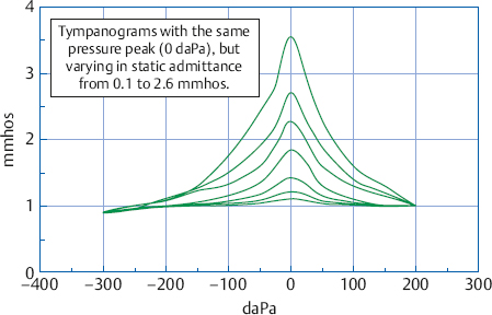
Fig. 7.6 Examples of tympanograms with static admittance values ranging from (top to bottom) 2.6, 1.7, 1.3, 0.9, 0.4, 0.2, to 0.1 mmho. These values are the distances in mmho between the height of the peaks and the ear canal value of 1.0 mmho at +200 daPa.
If we apply the classical tympanogram types to the examples in Fig. 7.6 we would categorize those having static admittance within the normal range as type A. The tympanogram with abnormally high admittance would be classified as either type AD or ADD. The two tympanograms with abnormally low admittance would be classified as AS, although the lowest one might be considered “flat” enough to be categorized as type B. Notice that the tympanograms in this group have peaks at 0 daPa, so that the type A categories are straightforward. If these tympanograms had peak pressures of perhaps –165 daPa, then they would all have been classified as type C, and the differences in static admittance would have been obscured. (A possible exception is the lowest one, which might have been classified as type B.) This issue emphasizes the idea that details can be lost if one makes the mistake of considering tympanograms only by their letter designations.
Tympanometric Gradient and Width
We see in Fig. 7.6 that the tympanogram peak becomes smaller as the static admittance becomes lower. If the admittance becomes low enough, then there will be no discernible peak, so that the tympanogram is described as flat. This is a common finding in ears with otitis media and cholesteatoma, where the static admittance may be as low as 0.06 or less (Jerger, Anthony, et al 1974). The flatness (versus peakedness) of a tympanogram can also be quantified by its gradient, which describes the relationship of its height and width. The gradient was originally calculated in terms of arbitrary units of compliance (Brooks 1969), as shown in Fig. 7.7a, and is determined as follows: (1) Draw a horizontal line where the width of the tympanogram is 100 mm H2O (or daPa). (2) Measure the height of the peak above this line (hp), as well as the total height (ht) of the tympanogram from its peak to its baseline. In the figure hp is 3.6 compliance units and ht is 8 units. (3) Find the gradient by dividing hp/ht, which is 3.6/8 = 0.45 in the figure. The same procedure can be used to calculate the gradient of absolute tympanograms, except that the heights are measured in terms of mmhos or ml.
Tympanometric gradients less than 0.2 are considered to be abnormally low (Nozza, Bluestone, Kardatzke, & Bachman 1992) and are associated with the presence of middle ear fluid (Brooks 1969; Paradise, Smith, & Bluestone 1976; Fiellau-Nikolajsen 1983; Nozza et al 1992).
Another way to quantify the flatness of a tympanogram is to determine the tympanometric width (Koebsell & Margolis 1986; ASHA 1997), which is simply the width of the tympanogram in daPa measured at 50% of its static acoustic admittance value. The method for determining tympanometric width is illustrated by the example in Fig. 7.7b. The static admittance value is measured at the tympanogram peak and is found to be 0.85 mmho in this example. We measure down 0.425 mmho from the peak because this distance is half the static value, and draw a horizontal line intersecting both sides of the tympanogram. Next, we draw vertical lines from these intersection points down to the x-axis. The tympanogram width is the distance between these two lines. In the example the tympanogram width is 80 daPa because the vertical lines cross the x-axis at –40 daPa and +40 daPa (which are 80 daPa apart).
Tympanometric widths that are too wide are associated with middle ear effusion, and normative data may be used to help determine when this is the case (e.g., Koebsell & Margolis 1986; Margolis & Heller 1987; Nozza, Bluestone, Kardatzke, & Bachman 1992, 1994; Silman, Silverman, & Arick 1992; Roush, Bryant, Mundy, Zeisel, & Roberts 1995; AAA 1997; ASHA 1997; Shahnaz & Polka 1997; De Chicchis, Todd, & Nozza 2000). Representative upper cutoff values for tympanometric width are 235 daPa for infants and 200 daPa for 1-year-olds through school-age children (ASHA 1997). Typical 90% normal ranges for adults are 51 to 114 daPa (Margolis & Heller 1987) and 48 to 134 daPa (Shahnaz & Polka 1997).
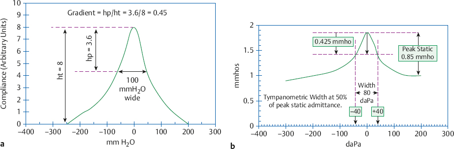
Fig. 7.7 Examples illustrating how to measure (a) tympanometric gradient (shown in terms of the arbitrary compliance units that were used by relative immittance bridges) and (b) tympanometric width.
Ear Volume
Tympanograms with extremely small or absent peaks are often referred to as essentially flat. These findings are usually attributed to extremely low middle ear admittance, and are typically associated with middle ear pathologies such as otitis media and cholesteatoma. However, we can reach this conclusion only if the volume (admittance at 226 Hz) measured at +200 daPa (or at –300 or –400 daPa) is attributable to the ear canal. If the volume is too large, then the flat tympanogram may be due to such causes as (1) a perforated tympanic membrane; (2) a patent myringotomy tube, if one is present; or (3) the absence of a hermetic seal. It is reasonable to consider the volume to be larger than normal when it exceeds 2.0 ml (mmhos) in children and 2.5 ml (mmhos) in adults (Van Camp et al 1986; Silman & Silverman 1991). On the other hand, the following causes are associated with volumes that are too small: (1) a clogged probe tip; (2) a probe tip that is pushed against the canal wall; (3) impacted cerumen or another obstruction in the ear canal; and (4) a clogged myringotomy tube if one is present. These cases are usually identified by volumes at or close to 0 ml (mmhos). Fig. 7.8 demonstrates how the flat tympanograms associated with tympanic membrane perforation, otitis media with effusion, and a clogged probe tip are differentiated on the basis of their ear canal volumes. It is very important to keep this issue in mind when tympanograms are classified by type because the letter designation does not account for the ear volume. For example, we could not attribute the type B tympanogram in Fig. 7.5 to middle ear effusion unless we also know the ear volume.
Tympanometric Peak Pressure
We know the pressure on the outer ear side of the eardrum because it is generated and measured using the air pump and manometer connected to the probe tip. In addition, we have learned that the tympanogram peak occurs when the same pressure exists on both sides of the tympanic membrane. Consequently, the ear canal pressure corresponding to the tympanogram peak is also an estimate of the pressure within the middle ear. Fig. 7.9 shows otherwise identical tympanograms with peak pressures of 0, –50, –150, and –250 daPa. Notice how increasingly negative tympanometric peak pressures are shown moving to the left of 0 daPa. Even though “tympanometric peak pressure” and “middle ear pressure” are often used interchangeably, we distinguish between the two terms here to point out that they are not always the same, especially when the patient has a flaccid tympanic membrane (Elner, Ingelstedt, & Ivarsson 1971; Renvall & Lidén 1978; Margolis & Shanks 1985).
Abnormally negative tympanometric peak pressures are associated with Eustachian tube disorders, which can occur either with or without the presence of middle ear fluid. The amount of negative pressure needed to consider the tympanometric peak pressure abnormally negative is not clearly identifiable in the literature. Suggested cutoff values vary widely, including values such as –25 daPa (Holmquist & Miller 1972), –30 daPa (Feldman 1975), –50 daPa (Porter 1972), –100 daPa (Jerger 1970; Jerger, Jerger, & Mauldin 1972; Jerger, Jerger, Mauldin, & Segal 1974; Fiellau-Nikolajsen 1983; Silman, Silverman, & Arick 1992), –150 daPa (Renvall & Lidén 1978; Davies, John, Jones, & Stephens 1988), –170 daPa (Brooks 1969), and –200 daPa (AAA 2012). In practice, –100 daPa appears to be a reasonable low cutoff value for tympanometric peak pressure. Lower pressures suggest the possibility of Eustachian tube dysfunction. Unfortunately, there does not seem to be a particular tympanometric peak pressure cutoff value that successfully distinguishes between the presence and absence of middle ear effusion. Several other tests of Eustachian tube function are described in the last section of this chapter.
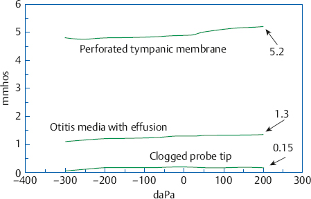
Fig. 7.8 Flat tympanograms from cases with tympanic membrane perforation (top), otitis media with effusion (middle), and a clogged probe tip (bottom). Ear canal volumes at +200 daPa are indicated for each.
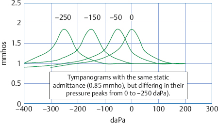
Fig. 7.9 Examples of tympanograms with tympanometric peak pressures of 0 daPa, –50 daPa, –150 daPa, and –250 daPa.
One can sometimes follow the course of recovery from a case of otitis media as tympanometric peak pressures that become progressively less negative over time (Feldman 1976). This course of events can be seen in stylized form by imagining that the series of tympanograms in Fig. 7.9 follows a sequence going from –250 daPa toward 0 daPa over a period of several days.
Unlike the situation for negative middle ear pressure, the significance of abnormally high positive peak pressures (e.g., > 50 daPa) is not clear. In spite of the extensive literature on tympanometry and middle ear pathology, only a few papers have reported positive pressures in some cases of otitis media (Paradise et al 1976; Feldman 1976; Ostergard & Carter 1981). In addition, positive peak pressure has also been associated with nonpathologic causes such as rapid elevator rides, crying, or nose blowing (Harford 1980).
Tympanogram Shape
Low-frequency probe tones like 226 Hz are mainly sensitive to changes in stiffness (or compliance). The shapes of most 226 Hz (220 Hz) tympanograms do not provide much information because they are usually single-peaked or flat. The infrequent exception is the presence of a notch in the tympanogram peak. Notched tympanograms are produced when mass becomes a significant component of the ear’s immittance, which occurs near and above its resonant frequency. For this reason notching is common with high-frequency probe tones, (e.g., 660 or 678 Hz) (Vanhuyse, Creten, & Van Camp 1975; Van Camp, Creten, van de Heyning, Decraemer, & Vanpeperstraete 1983; Van Camp et al 1986; Wiley, Oviatt, & Block 1987). Notching of the 226 Hz tympanogram is abnormal because it means that something is causing mass to play a greater than normal role in the ear. These changes can be produced by a scarred or flaccid tympanic membrane (even in an otherwise normal ear), as well as abnormalities such as ossicular discontinuities (which produce substantial hearing losses). Recall that these are the aberrations associated with type D and E tympanograms.
Vascular Pulsing
Although most tympanograms are smooth, they sometimes have regular ripples or undulations that are synchronized with the patient’s pulse, which is their origin. Medical referral is indicated when vascular pulsing is present on the tympanogram because it tends to occur in patients with glomus jugulare tumors (Feldman 1976).
678 Hz (660 Hz) Tympanograms
“High-frequency” tympanograms are obtained with probe tones higher than the traditional “low-frequency” 226 Hz (or 220 Hz) probe tone. The “high-frequency” probe tone is usually 678 Hz (or 660 Hz). The combined use of 226 Hz and 678 Hz tympanograms is sometimes called multiple frequency (or multifrequency) tympanometry. However, this term is also used to describe various tympanometric methods that involve testing at many frequencies to arrive at the resonant frequency of the ear and other measures. Abnormally high resonant frequencies are associated with stiffening disorders, such as otosclerosis, whereas abnormally low resonant frequencies are associated with disorders that increase the mass component of the system, like ossicular discontinuity. The details of these and other advanced approaches are not covered here, but the interested student will find many readily available sources (e.g., Shanks, Lilly, Margolis, Wiley, & Wilson 1988; Shanks & Shelton 1991; Hunter & Margolis 1992; Margolis & Goycoolea 1993; Shahnaz & Polka 1997).
Separate tympanograms are obtained for susceptance (B) and conductance (G) when testing at 678 Hz (or 660 Hz) instead of a single admittance (Y) tympanogram. Depending on the instrumentation used, the B and G tympanograms may be obtained simultaneously (which is preferred), or they may be done one after the other. In either case, the interpretation is easier when they are plotted on the same tympanogram form.
Normal 678 (660) Hz Tympanograms
In contrast to 226 Hz tympanograms, 678Hz (660 Hz) B-G tympanograms are interpreted on the basis of their shapes and configurations (or morphology). There are four types of normal 678 Hz B-G tympanograms (Vanhuyse et al 1975; Van Camp et al 1983, 1986; Wiley et al 1987). They are named on the basis of the number of positive and negative peaks and must also meet a criterion for tympanogram width.
The first normal type of 678 Hz tympanogram is called 1B1G because there is one peak for the B tympanogram and one peak for the G tympanogram (Fig. 7.10a). The other three normal variations involve notches on one or both of the tympanograms. The second normal type has a notched peak on the B tympanogram and a single peak on the G tympanogram. Notice that the notch on the B tympanogram can be viewed as two positive peaks with a negative peak between them. The convention is to count these “peaks” or “extrema.” Thus, this normal variation is called 3B1G because B has three peaks and G has one peak (Fig. 7.10b). The third normal variation is called 3B3G because there are three peaks on both tympanograms (Fig. 7.10c). The last type of normal 678 Hz (or 660 Hz) configuration is called 5B3G because it has five peaks on the B tympanogram and three peaks on the G tympanogram (Fig. 7.10d). In addition to having a maximum of five peaks for B and three peaks for G, the distance between the outermost peaks of normal 678 Hz B-G tympanograms should be (1) ≤ 75 daPa wide for 3B3G tympanograms and ≤ 100 daPa for 5B3G tympanograms, and (2) narrower for the G tympanogram than for the B tympanogram. Table 7.4 shows the percentages of normal adults with each of the 678 Hz B-G tympanogram types.
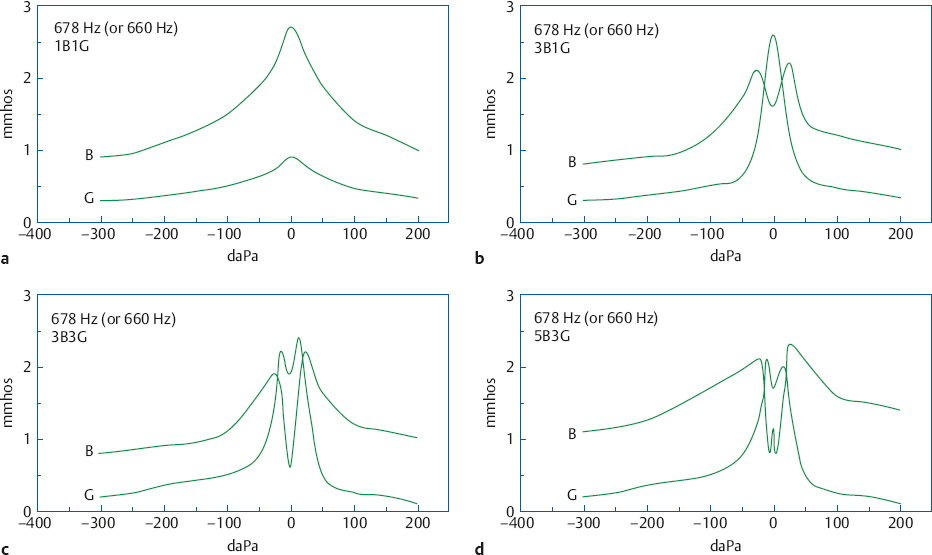
Fig. 7.10 Illustrative examples of normal B-G tympanograms obtained at 678 Hz (or 660 Hz): (a) 1B1G, (b) 3B1G, (c) 3B3G, and (d) 5B3G.
Stay updated, free articles. Join our Telegram channel

Full access? Get Clinical Tree


