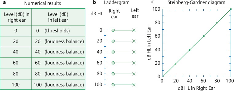
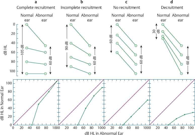
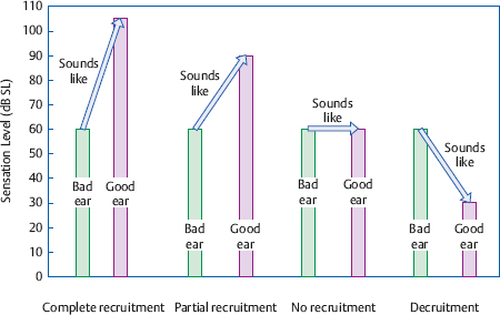
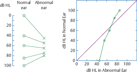
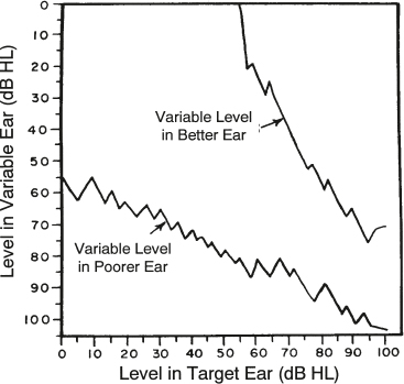
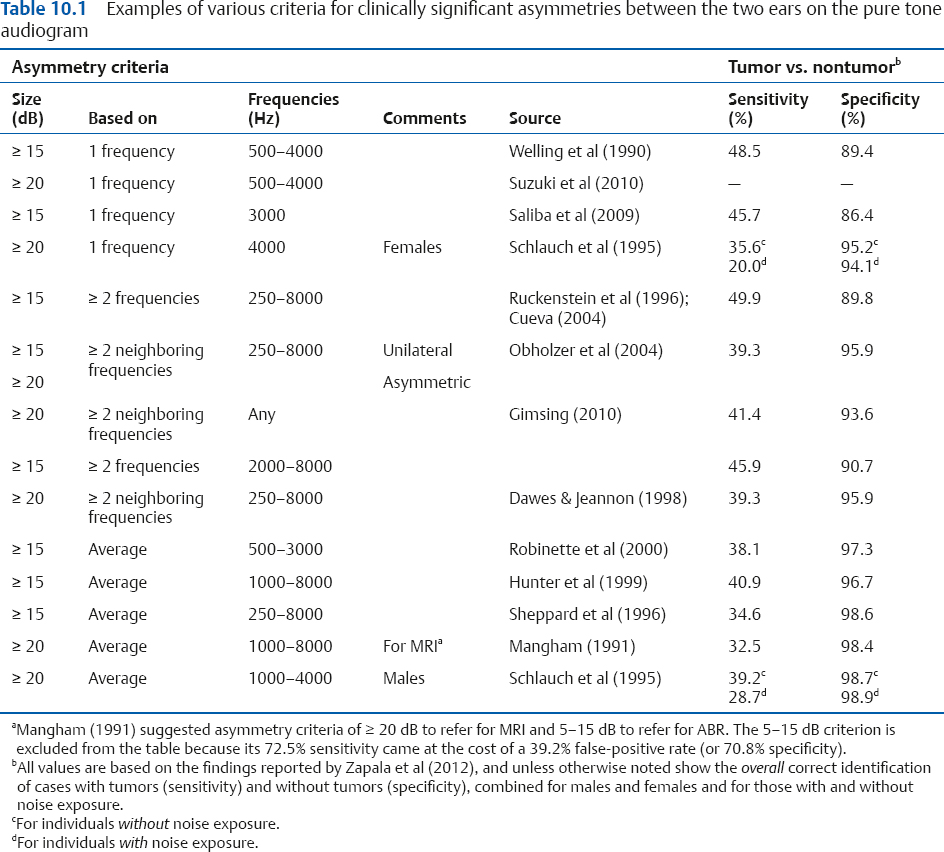
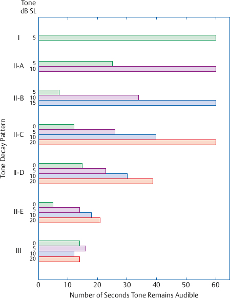
10 Behavioral Tests for Audiological Diagnosis

In this chapter, we will briefly consider whether asymmetries between the right and left ears on the pure tone audiogram help us to identify retrocochlear disorders; after which we will consider the classical site-of-lesion tests. As discussed in Chapter 6, terms like acoustic neuroma or tumor, vestibular schwannoma, and eighth nerve tumor will be used interchangeably. Following the traditional tests, we will cover the behavioral measures used to identify cochlear dead regions and some aspects of the assessment of central auditory processing disorders.

Asymmetries between the Ears

Recall from Chapters 5 and 6 that cochlear and eighth nerve lesions cannot be distinguished from one another based on the pure tone audiogram. In fact, any degree and configuration of hearing loss can be encountered in patients with retrocochlear pathology (e.g., Johnson 1977; Gimsing 2010; Suzuki, Hashimoto, Kano, & Okitsu 2010). In spite of this, a significant difference between the ears is a very common finding in patients with acoustic tumors (e.g., Matthies & Samii 1997), so that the index of suspicion is raised when an asymmetry is found. Although we will be focusing here on asymmetries in the pure tone audiogram, it is important to stress that other asymmetries also raise the flag for ruling out retrocochlear pathology. Unilateral tinnitus (e.g., Sheppard, Milford & Anslow 1996; Dawes & Jeannon 1998; Obholzer, Rea, & Harcourt 2004; Gimsing 2010) and differences in speech recognition scores between the ears (e.g., Welling, Glasscock, Woods, & Jackson 1990; Ruckenstein, Cueva, Morrison, & Press 1996; Robinette, Bauch, Olsen & Cevette 2000) are among the other examples of asymmetries that become apparent early in the evaluation process.

However, many patients without retrocochlear pathology often have some degree of difference between their ears, as well; and there can be disagreement about whether a hearing loss is symmetrical or asymmetrical even among expert clinicians (Margolis & Saly 2008). It is therefore desirable to have criteria for identifying when a sensorineural hearing loss involves a clinically significant asymmetry. Thus, it is not surprising that various criteria have been suggested for identifying asymmetries in the pure tone audiogram that are clinically significant. Many of these criteria are summarized in Table 10.1, although other kinds of approaches using mathematical and statistical techniques have also been developed (e.g., Nouraei, Huys, Chatrath, Powles, & Harcourt 2007; Zapala et al 2012).

Some of the methods in Table 10.1 use an inter-ear difference of ≥ 15 dB as the criterion for a clinically significant asymmetry, while others use require ≥ 20 dB. They also differ with respect to which frequencies are considered, how many of them are involved, and how the differences are calculated. The first two methods in the figure consider a difference between the ears to be clinically significant even if it occurs at just one frequency between 500 and 4000 Hz; and each of the next two considers only one specific frequency. The third set of methods require an asymmetry to be present for at least two frequencies in a range, but differ in terms of whether they can be any two frequencies or only ones that are adjacent to one another. Finally, the last group of methods compare an average of the thresholds for a certain range of frequencies. Also notice that a few methods use different criteria based on gender, on whether the hearing loss is unilateral versus bilateral but asymmetrical, and even on whether the next step in the process would be magnetic resonance imaging (MRI) or auditory brainstem responses (ABR). So, with all these differences, which criteria should be used?

At least part of the answer to this question is provided in the last two columns of the table, which are based on the findings by Zapala et al (2012) for patients with hearing losses that were known to be either medically benign or associated with vestibular schwannomas. The sensitivity (also known as the hit rate) column shows the percentage of patients who had vestibular schwannomas who were correctly identified by the criteria. In contrast, the specificity column shows the percentage of patients who did not have tumors and who were correctly identified by the criteria. For example, the criteria by Welling et al (1990) had 49.5% sensitivity and 89.4% specificity. This means that their method correctly identified 49.5% of the patients with tumors and 89.4% of those without tumors. This also means that 100 – 49.5 = 50.5% of the patients with tumors were missed by the method (false negatives), and that it also incorrectly flagged 100 – 89.4 = 10.6% of those who did not have tumors (false positives). Overall, we see that these provide up to ~ 50% specificity and roughly 14% specificity. Somewhat better performance can be achieved with a statistical approach that allows the clinician to estimate the sensitivity and false positive rate for a given patient (Zapala et al 2012). This method uses the average difference between the ears at 250 to 4000 Hz (including 3000 Hz) and includes adjustments for the patient’s age, gender, and noise exposure history.

Which method is “best”? The answer to this question depends on how the comparison is made, and provides a convenient opportunity to introduce some useful concepts.

One way to identify the optimal method is to find the one that has the highest sensitivity and the highest specificity. In these terms, the overall topperforming criteria in the table were ≥ 15 dB for ≥ 2 frequencies between 250 and 8000 Hz (Ruckenstein et al 1996; Cueva 2004) with 49.9% sensitivity and 89.8% specificity, and ≥ 15 dB for 1 frequency between 500 and 4000 Hz (Welling et al 1990) with 48.5% sensitivity and 89.4% specificity.¹

Another way to compare the methods is to graph the hit rate against the false alarm rate.² (We will bypass the details, but interested students will want to know that this approach comes from the theory of signal detection, and the plot is called a receiver operating characteristic or ROC curve [see, e.g., Gelfand 2010].) With this approach, Zapala et al (2012) found that their statistical method was the most effective method for distinguishing vestibular schwannomas from medically benign cases, followed by a close tie between ≥ 15 dB for the 250 to 8000 Hz average (Sheppard et al 1996) and ≥ 15 dB for the 500 to 3000 Hz average ( Robinette et al 2000).

The picture that emerges is that a significantly asymmetrical hearing loss provides up to ~ 50% sensitivity along with good specificity, and that the criteria just highlighted seem to be reasonable choices for use. Considering the limited sensitivity and high specificity of the criteria, a referral to rule out retrocochlear pathology is certainly warranted when a significant asymmetry is identified.

¹ A noticeable exception occurred for women with a history of noise exposure, for whom sensitivity was 40% with the Welling et al (1990) method compared with 30% for the Ruckenstein et al (1996) criteria (Zapala et al 2012).

² Because of the high level used, a 90 dB SPL broadband masking noise is presented to the opposite ear.

A common thread among many of the traditional behavioral tests for distinguishing cochlear and retrocochlear disorders is the perception of intensity and how it is affected by pathology. We shall see, however, that the ability of these kinds of tests to confidently separate cochlear and retrocochlear disorders has actually been rather disappointing, and their use has decreased over the years (Martin, Champlin, & Chambers 1998). In spite of this, we will cover these tests in some detail not just because one will find the need to use them from time to time, but also because this knowledge provides the future clinician with (a) insight into the nature of hearing impairment, (b) familiarity with various approaches used to assess auditory skills, and (c) the all-important foundation needed for understanding the literature in the field.

Threshold Tone Decay Tests

A continuous tone sounds less loud after it has been on for some time compared with when it was first turned on, or it may fade away altogether. The decrease in the tone’s loudness over time is usually called loudness adaptation, and the situation in which it dies out completely is called threshold adaptation or tone decay. Adaptation is due to the reduction of the neural response to continuous stimulation over time, and is common to all sensory systems (Marks 1974). Adaptation per se is a normal phenomenon, but excessive amounts of adaptation reflect the possibility of certain pathologies. It is for this reason that adaptation tests are often used as clinical site-of-lesion tests.

Most clinical adaptation procedures are threshold tone decay tests, which measure adaptation in terms of whether a continuous tone fades away completely within a certain amount of time, usually 60 seconds. The patient’s task is easily understood in terms of these typical instructions: “You will hear a continuous tone for a period of time, which might be a few seconds or a few minutes. Raise your finger (or hand) as soon as the tone starts and keep it up as long as the tone is audible. Put your finger down whenever the tone fades away. Pick it up again if the tone comes back, and hold it up as long as you can still hear it. It is very important that you do not say anything or make any sounds during this test because that would interrupt the tone. Remember, don’t make any sounds, keep your finger raised whenever you hear the tone, and down whenever you don’t hear it.” Because the patient may be holding his hand or finger up for some time, it is a good idea to have him support his elbow on the arm of his chair. Many audiologists have the patient press and release a response signal button instead of holding up and lowering his finger or hand.

Carhart (1957) suggested that tone decay tests (TDTs) be administered to each ear at 500, 1000, 2000, and 4000 Hz, but most audiologists select the frequencies to be tested on a patient-by-patient basis. Both ears should be tested at each frequency selected because this permits the clinician to compare the two ears as well as to determine whether abnormal tone decay is present bilaterally. Of course, each ear is tested separately.

Carhart Tone Decay Test

In the Carhart threshold tone decay test (1957), a test tone is presented to the patient at threshold (0 dB SL) for 60 seconds. If the patient hears the tone for a full minute at the initial level, then the test is over. However, if the patient lowers his finger, indicating that the tone faded away before 60 seconds have passed, then the audiologist (1) increases the level by 5 dB without interrupting the tone, and (2) begins timing a new 60-second period as soon as the patient raises his hand. If the tone is heard for a full minute at 5 dB SL, then the test is over. However, if the tone fades away before 60 seconds are up, then the level is again raised 5 dB and a new minute is begun. This procedure continues until the patient is able to hear the tone for 60 seconds, or until the maximum limits of the audiometer are reached.

Tone decay test results are expressed as the amount of tone decay, which is simply the sensation level at which the tone was heard for 60 seconds. For example, if the tone was heard for 1 minute at threshold, then there would be 0 dB of tone decay; and if the tone was heard for 60 seconds at 5 dB SL, then there was 5 dB of tone decay. Similarly, if the tone could not be heard for a full minute until the level was raised to 45 dB SL, then there would be 45 dB of tone decay.

Normal individuals and those with conductive abnormalities are expected to have little or no threshold adaptation. Cochlear losses may come with varying degrees of tone decay, which may range up to perhaps 30 dB, but excessive tone decay of 35 dB or more is associated with retrocochlear pathologies (Carhart 1957; Tillman 1969; Morales-Garcia & Hood 1972; Olsen & Noffsinger 1974; Sanders, Josey, & Glasscock 1974; Olsen & Kurdziel 1976). Thus, if the TDT is viewed as a test for retrocochlear involvement, then ≤ 30 dB of tone decay is usually interpreted as “negative,” and > 30 dB of tone decay is “positive.”

Tone decay test outcomes should be documented separately for each ear in terms of the number of decibels of tone decay at each frequency tested, to which one might add an interpretation (such as “positive” or “negative”). One should never record “positive” or “negative” without the actual results. You can always figure out whether a result was positive or negative from the amount of tone decay, but you could never go back and deduce the actual amount of tone decay from a record that says only “positive” or “negative.” These points apply to all diagnostic procedures.

Olsen-Noffsinger Tone Decay Test

The Olsen-Noffsinger tone decay test (1974) is identical to the Carhart TDT except that the test tone is initially presented at 20 dB SL instead of at threshold. Beginning at 20 dB SL is desirable for several reasons. It makes the test simpler for the patient to take because a 20 dB SL test tone is much easier to detect than one given at threshold. It is also easier to distinguish it from any tinnitus that the patient may have. In addition, starting the test at 20 dB SL can shorten the test time by as much as 4 minutes for every frequency tested. Reducing the test time makes the experience less fatiguing for the patient and saves clinician time, which is always at a premium. The Olsen-Noffsinger modification relies on the premise that amounts of tone decay up to 20 dB on the Carhart TDT are interpreted as negative. Thus, omitting the test trials that would have been given at 0 to +15 dB SL should not change any diagnostic decisions. It has been found that the Carhart and Olsen-Noffsinger procedures yield similar results in terms of when the results are positive versus negative (Olsen & Noffsinger 1974; Olsen & Kurdziel 1976).

The outcome of the Olsen-Noffsinger TDT is recorded as follows: If the patient hears the initial (20 dB SL) test tone for a full minute, then one records the results as “≤ 20 dB tone decay.” Greater amounts of tone decay are recorded in the same way as for the Carhart TDT.

The Olsen-Noffsinger TDT Is sometimes misconstrued as a tone decay “screening” test because most patients are able to hear the initial test tone for the full 60 seconds. It should be stressed that the reason why many patients do not have to be tested beyond the 20 dB SL starting level is simply that they do not have more than 20 dB of tone decay. One should remember that the Olsen-Noffsinger is a full-fledged TDT that yields the actual amount of significant tone decay > 20 dB, just like the Carhart procedure.

Other Modifications of the Carhart Tone Decay Test

There are several other modifications of the Carhart TDT of which the student should be aware. The Yantis (1959) modification begins testing at 5 dB SL instead of at threshold. This modification is so commonly used that it is not distinguished from the Carhart by most clinicians. Sorensen’s (1960, 1962) modification requires the patient to hear the test tone for 90 seconds instead of 60 seconds, and is performed only at 2000 Hz. This procedure is rarely used.

The Rosenberg (1958, 1969) modified tone decay test begins like the Carhart test but lasts only 60 seconds from start to finish. If the patient hears the tone for 60 seconds at threshold, then the test is over and there is 0 dB of tone decay. If the tone fades away before the end of one minute, then the clinician does the following: As with the Carhart TDT, she increases the intensity in 5 dB steps without interrupting the tone until the patient raises his hand. Every time the patient lowers his hand, the audiologist again raises the tone in 5 dB steps until the patient hears the tone again, and so on. However, unlike the Carhart TDT, she does not begin timing a new minute with every level increment. Instead, the clock keeps running until a total of 60 seconds has elapsed since the tone was originally turned on. The amount of tone decay is the sensation level reached at the end of 60 seconds. For example, if the threshold was 35 dB HL, the tone starts at this level and one begins timing for 60 seconds. If the attenuator has been raised by a total of 25 dB to 60 dB HL at the end of one minute, then there has been 25 dB of tone decay. Notice that the Rosenberg test ignores how long the tone was actually heard at any given level.

Green’s (1963) modified tone decay test involves administering the Rosenberg 1-minute test with a significant change in the instructions. The patient is told to lower his hand completely if the tone fades away and to lower his hand partially if the tone loses its tonal quality (even though it might still be audible). The modified instructions are based on the observation that some patients with retrocochlear pathologies hear a change in the character of the tone in which it loses it tonal quality, becoming noise-like, before its audibility is completely lost (Pestalozza & Cioce 1962; Sorensen 1962; Green 1963). This phenomenon is called atonality or tone perversion (Parker & Decker 1971).

Owens Tone Decay Test

Owens (1964a) introduced a modification of a tone decay procedure originated by Hood (1955). Unlike the Carhart test and its modifications, which concentrate on the amount of adaptation, the Owens tone decay test focuses upon the pattern of tone decay. The test begins by presenting a continuous test tone at 5 dB SL. As with the Carhart TDT, the Owens test ends if the patient hears the tone for 60 seconds at this initial level. However, if the tone fades away before 60 seconds, the tone is turned off for a 20-second rest (recovery) period. After the 20-second rest, the tone is reintroduced at 10 dB SL (i.e., 5 dB higher), and a new 60-second period begins. If the tone is heard for a full minute at 10 dB SL, then the test is over. However, if the tone fades away before a full minute, then the tone is turned off for another 20-second rest period, after which it is given again at 15 dB SL. The same procedure is followed for the 15 dB SL tone. If necessary, the tone is presented for another 1-minute period at 20 dB SL, but this is the last level tested regardless of whether the tone is heard for 60 seconds or less. The audiologist records how many seconds the tone was heard at each of the levels presented, and the test is interpreted in terms of the pattern of how many seconds the tone was heard at each of the four test levels.

Fig. 10.1 shows the various patterns (types) of tone decay described by Owens (1964a). The type I pattern involves being able to hear the initial (5 dB SL) tone for a full minute, and is associated with normal ears and those with cochlear impairments.

There are five type II patterns, called II-A through II-E. The type II patterns share two characteristics: (1) the tone fades away before 60 seconds for at least the lowest sensation level, and (2) the tone is heard progressively longer at increasingly higher sensation levels. The tone is finally heard for a full minute at 10 dB SL in type II-A, at 15 dB in type II-B, and at 20 dB SL in type II-C. In the type II-D pattern, the tone fades away in less than a minute at all four sensation levels, but it does remain audible for appreciably longer periods of time with each successively higher sensation level. Cochlear impairments are most commonly associated with types II-A through II-D.

In the type II-E pattern each 5 dB rise in sensation level produces only a small increase in how long the tone is heard (averaging 4 to 7 seconds per 5 dB level). This pattern is found in either cochlear or retrocochlear abnormalities.

The type III pattern is principally associated with retrocochlear disorders. Here, increasing the sensation level does not cause the tone to be heard for longer periods of time.

Rate of Tone Decay

Wiley and Lilly (1980) proposed a modification of the Owens TDT in which (1) the rest period between tones is reduced to 10 seconds, and (2) the test level continues to be raised until the tone remains audible for a full minute (or the audiometer’s maximum level is reached). This modification allowed them to distinguish between the rates of tone decay in the two ears of a patient who had a cochlear disorder in one ear and an acoustic tumor in the other ear. The importance of looking at the rate of tone decay was also shown by Silman, Gelfand, Lutolf, and Chun (1981) in a patient whose hearing loss was so severe that the Owens TDT was the only usable tone decay method.

Overall Assessment of Threshold Tone Decay Tests

Tone decay appears to be the only classical site-oflesion technique that is still routinely used by a majority of audiologists (Martin et al 1998). Several studies have compared the accuracy of threshold adaptation tests as indicators of retrocochlear pathology (e.g., Parker & Decker 1971; Olsen & Noffsinger 1974; Sanders, Josey, & Glasscock 1974). Overall, they have shown the Carhart-type TDTs are most sensitive procedures. This appears to hold true whether the test begins at threshold, 5 dB SL (Yantis 1959), or 20 dB SL (Olsen & Noffsinger 1974). This kind of TDT is thus the one of choice, with the Olsen-Noffsinger modification being the most efficient. The Owens TDT is particularly valuable when the severity of a hearing loss makes it impossible to determine the amount of tone decay using the Carhart or similar procedures (Silman et al 1981). In contrast, the Rosenberg 1-minute TDT is not as effective at identifying retrocochlear lesions as the Carhart, Olsen-Noffsinger, or Owens procedure (Parker & Decker 1971; Olsen & Noffsinger 1974) and is not recommended.

Green’s modification of the Rosenberg TDT has not been compared with other tests that do not use the atonality criterion. It is not clear whether atonality per se should be used as a criterion for tone decay testing because little if any research actually addresses this issue. More tone decay can be obtained when the patient responds to either atonality or inaudibility compared with inaudibility alone. However, the experience of the author and his colleagues (e.g., Silman & Silverman 1991) has been that using the atonality criterion increases the number of false-positive TDT results, and this is especially problematic when testing elderly patients. Even though several earlier papers suggested accounting for the loss of tonal quality (e.g., Sorenson 1962; Pestalozza & Cioce 1962; Flottorp 1964; Johnson 1966; Sung, Goetzinger, & Knox 1969; Olsen & Noffsinger 1974), it appears that only ~ 10% of audiologists use the atonality criterion (Martin, Woodrick Armstrong, & Champlin 1994).

As a group, threshold TDTs correctly identify retrocochlear lesions among anywhere from 64 to 95% of the cases, and correctly classify non-retrocochlear disorders ~ 77 to 96% of the time (Owens 1964a; Gjaevenes & Söhoel 1969; Tillman 1969; Olsen & Noffsinger 1974; Sanders et al 1974; Olsen & Kurdziel 1976; Antonelli, Bellotto, & Grandori 1987; Josey 1987). Part of this variability comes from differences in which tone decay tests were used and how they were administered and interpreted, and also from differences in the patient populations. Turner, Shepard, and Frazer (1984) have shown that TDT results are correct in an average of 70% of retrocochlear cases and 87% for ears that do not have retrocochlear lesions, across studies.

Suprathreshold Adaptation Test

Jerger and Jerger (1975a) suggested a tone decay test performed at high levels instead of beginning at threshold, called the suprathreshold adaptation test (STAT). Here, a continuous test tone lasting a total of 60 seconds is presented at 110 dB SPL.² (This corresponds to ~ 105 dB HL when the test is done at 1000 Hz, and to 100 dB HL when testing at 500 Hz or 2000 Hz.) As with threshold tone decay tests, the patient is told to keep her hand raised as long as she hears the tone, and to lower her hand if it fades away completely. If the high-intensity tone is heard for the full minute, then the test is over and the result is negative. If the tone fades away before 60 seconds are up, then the patient is retested with a pulsing tone for confirmatory purposes. If the patient keeps her hand up for the full 60 seconds in response to the pulsing tone, then her failure to keep responding to the continuous tone is attributed to abnormal adaptation. The test is thus confirmed to be positive, suggesting a retrocochlear disorder. However, if she fails to respond to the pulsing tone for 1 minute, then the test result is not considered to be valid because tone decay should not occur with a pulsed tone. The correct identification rates for cochlear and retrocochlear cases, respectively, are 100% and 45% when the STAT is done at 500 and 1000 Hz, 95% and 54% at 500 to 2000 Hz, and 13% and 70% at 500 to 4000 Hz (Jerger & Jerger 1975a; Turner et al 1984).

Loudness Recruitment and Loudness Balance Testing

Loudness Recruitment

We all have had the experience of being told to “speak up” by a hearing-impaired relative. Upon complying with this request, we are then told to “stop shouting.” This common experience reveals an important facet of many cochlear impairments: Even though more intensity (i.e., a higher than normal HL) is needed for a sound to be heard, once the sound is raised above this elevated threshold, the now higher-intensity sound is as loud to the patient as it would be to a normal-hearing person. Consider a normal person whose threshold for a tone is 0 dB HL and a patient whose threshold is 50 dB HL for the same tone. If the tone is raised to 80 dB HL, it will now be 80 dB above the normal person’s threshold but only 30 dB above the patient’s threshold. Yet the tone will sound as loud to the patient (at 30 dB SL) as it does to the normal individual (at 80 dB SL). For this patient, the 30 dB level increase was perceived as an increase in loudness by an amount that took an 80 dB level increase for the normal person. In other words, the patient has experienced an abnormally rapid growth of loudness. This is called loudness recruitment.

When there is a sensorineural hearing loss, loudness recruitment is associated with a cochlear site of lesion, whereas the absence of loudness recruitment is associated with retrocochlear pathologies (Dix, Hallpike, & Hood 1948; Hallpike & Hood 1951, 1959; Jerger 1961; Hallpike 1965; Davis & Goodman 1966; Hood 1969; Priede & Coles 1974; Coles & Priede 1976).

Alternate Binaural Loudness Balance (ABLB) Test

The nature of the alternate binaural loudness balance (ABLB) test (Fowler 1936) is described by its name. A tone is presented alternately between the two ears (binaurally). The level of the tone stays the same in one ear (the “fixed” ear), but is varied up and/or down in the other ear (the “variable” ear), as shown schematically in Fig. 10.2. The patient reports when the tone sounds louder in the right ear, when it is louder in the left ear, and when it sounds equally loud in both ears. We say that a loudness balance has been obtained when the tones sound equally loud in both ears. The tester then records the two levels (in dB HL) where the loudness balance occurred.

² Because of the high level used, a 90 dB SPL broadband masking noise is presented to the opposite ear.

Let us see what happens when the ABLB is given to a normal-hearing person who has the same thresholds in both ears. The results of a series of loudness balances at the same frequency in 20 dB intervals are shown in the left panel of Fig. 10.3. We assume that 0 dB HL in the right ear and 0 dB HL in the left ear are equally loud because they are both at threshold. Moving on to the loudness balances themselves, notice that 20 dB HL in the right ear sounded as loud as 20 dB HL in the left ear, 40 dB HL in the right ear was just as loud as 40 dB HL in the left ear, etc. Although ABLB results can be recorded numerically, it is more convenient to show them diagrammatically. The diagram in the middle panel of Fig. 10.3 is called a laddergram for obvious reasons. Hearing level is shown going down the y-axis just as on an audiogram. For each loudness balance, we draw a circle at the hearing level in the right ear and an X at the hearing level for the left ear, and then join the two symbols with a line to show they are equally loud. The horizontal lines (“rungs”) indicate that equal loudness occurs at the same intensity for both ears. We can also show the results on a Steinberg-Gardner plot like the one in the right panel of the figure. Here, each point shows the coordinates of the levels in the two ears that sound equally loud. In this example, all of the points fall along a diagonal line because there was a one-to-one relationship between the equally loud levels in the two ears. Whenever the points fall along this 45° line, it means that equal intensities sound equally loud.

Types of Recruitment

Complete recruitment is shown in Fig. 10.4a. Here, even though the thresholds are 0 dB HL and 45 dB HL, equal loudness is eventually obtained when both ears receive 105 dB HL. In practice, recruitment is generally considered complete if equal loudness occurs at equal hearing levels (dB HL) ± 10 dB (Jerger 1962). This is shown by the flattening of the rungs on the laddergram. In this example, a 60 dB rise (from 45 to 105 dB HL) in the abnormal ear sounds like a 105 dB rise (from 0 to 105 dB HL) in the normal ear. In terms of sensation level, 60 dB SL in the bad ear is experienced as being just as loud as 105 dB SL in the good ear (Fig. 10.5a).

Complete recruitment is easily seen on the Steinberg-Gardner plot (Fig. 10.4a), which plots the level in the abnormal ear on the x-axis and the equally loud level in the good ear on the y-axis. The normal one-to-one loudness-growth relationship is shown by a 45° line for comparison purposes. Any points that fall on this diagonal indicate that equal intensities sound equally loud. The plot of the test results begins 45 dB to the right (i.e., x = 45, y = 0) because the thresholds are 45 dB in the abnormal ear and 0 dB in the normal ear, but it rises at a sharp angle and eventually meets the 45° line at the point corresponding to 105 dB HL in both ears. The steeply rising line on the Steinberg-Gardner diagram gives a clear picture of what we mean when we say that recruitment is an abnormally rapid growth of loudness. As already pointed out, complete recruitment suggests a cochlear site of lesion.

Some patients with Meniere’s disease may exhibit a special case of recruitment in which the loudness in the abnormal ear not only catches up with the normal ear, but actually overtakes it (Dix et al 1948; Hallpike & Hood 1959; Hood 1977). This finding is called hyper-recruitment (or over-recruitment), and is shown in Fig. 10.6. Hyper-recruitment is revealed on the laddergram by rungs that first flatten and then reverse direction. In this example, 85 dB HL in the abnormal ear actually sounds as loud as 100 dB HL in the normal ear. This is shown on the Steinberg-Gardner diagram when the line that shows the patient’s equal loudness judgments crosses above the diagonal line. One should note that hyper-recruitment is something of a controversial issue, and the likelihood of finding it seems to be affected by how the ABLB test is performed (Hood 1969, 1977; Coles & Priede 1976).

Incomplete (or partial) recruitment occurs when the results fall between complete recruitment and no recruitment (discussed below). This is shown as a partial flattening of the laddergram or by a line that rises toward but does not quite reach the diagonal on the Steinberg-Gardner plot. An example is shown in Fig. 10.4b and Fig. 10.5b. Audiologists are inconsistent about how they interpret incomplete recruitment, and it is not surprising that its diagnostic value has been questioned (Priede & Coles 1974).

No recruitment occurs when the relationship between the levels at the two ears is the same for the loudness balances as it is at threshold. An example is shown in Fig. 10.4c and Fig. 10.5c. Here, the same 45 dB spread that exists between the left and right thresholds is also found for each of the loudness balances. This is seen as parallel lines on the laddergram. The situation is even clearer on the Steinberg-Gardner plot. In spite of the threshold difference between the ears, the line showing equally loud levels rises at a 45° angle just like the normal line. This shows that the spread between the two ears is maintained at high levels. It also means that a 20 dB increase in the abnormal ear sounds just as loud as a 20 dB increase in the normal ear; that is, loudness is growing at the same rate with increasing intensity in both ears. Consequently, loudness must be growing at the normal rate in the abnormal ear. As a practical guideline, one might say that there is no recruitment if equal loudness occurs at equal sensation levels (dB SL) ± 10 dB (Jerger 1962).

No recruitment is the expected result when the loss in the abnormal ear is conductive. In fact, Fowler (1936) originally conceived of the ABLB as a test to distinguish between otosclerosis (a conductive disorder) and sensorineural hearing losses. However, the ABLB is not used with conductive losses because its actual purpose is to help to distinguish between cochlear and retrocochlear disorders. Thus, finding no recruitment in a case of unilateral sensorineural loss is the same as failing to argue in favor of a cochlear disorder. By inference, this would lead us to suspect retrocochlear pathology.

In some cases, loudness grows at a slower than normal rate as intensity increases in the abnormal ear. This is called decruitment (Davis & Goodman 1966) or loudness reversal (Priede & Coles 1974) and is associated with retrocochlear pathology. In the example in Fig. 10.4d, 105 dB HL in the bad ear sounds only as loud as 30 dB HL in the good ear. In other words, 60 dB SL in the abnormal ear sounds like only 30 dB SL in the normal ear (Fig. 10.5d). In effect, loudness is lost rather than gained as intensity is raised.

ABLB Testing Approaches

Different procedures have been suggested for administering the ABLB. In Jerger’s (1962) protocol, the tone alternates between the ears automatically every 500 milliseconds (as in Fig. 10.2), with the fixed level in the abnormal ear and the variable signal in the normal ear. The patient changes the intensity of the tone in the variable ear using the method of adjustment (see Chapter 3) until it sounds equal in loudness to the tone in the fixed ear. Loudness balances are made at 20 dB intervals above the bad ear’s threshold, and are plotted on a laddergram.

One should note that because the tone alternates between the two ears every 500 milliseconds, it will be off for 500 milliseconds in each ear. This off-time ensures that the test tones will not be subject to adaptation. This requirement is met if the tone is off for at least a certain critical off-time, which is ~ 200 to 250 milliseconds (Dallos & Tillman 1966; Jerger & Jerger 1966; Tillman 1966).

Hood (1969, 1977) suggested manual control over the presentation of the tones according to the method of limits (see Chapter 3), using the good ear as the fixed-level ear, and plotting the results on a Steinberg-Gardner diagram. Others have suggested presenting the fixed-level tone to the bad ear and testing according to Hood’s method (Priede & Coles 1974; Coles & Priede 1976), or randomizing the use of the good and bad ears as the fixed-level ear under computer control (Fritze 1978).

Actual ABLB techniques vary widely among audiologists, many of whom use hybrid methods. For example, one might use automatically alternating tones with the fixed level in the bad ear, employ a modified method of limits or bracketing, and have the patient respond with hand signals, or by saying “right,” “left,” or “equal.”

An interesting ABLB modification by Miskolczy-Fodor (1964) uses the Bekesy tracking method (see below) to keep the level in the variable ear equally loud as the one in the reference ear, and the results are automatically plotted on paper. Fig. 10.7 shows an example. Two sets of results must be combined for accurate loudness balances with this method, one using the good ear as the reference and one using the bad ear (Carver 1970; Gelfand 1976). Otherwise, it over- or underestimates the loudness balance points. Other variations have also been reported (Sung & Sung 1976).

Stay updated, free articles. Join our Telegram channel

Join