(31.1)
Due to a double-pass (reflection imaging) geometry in OCT, the system PSF, h(x, y, z; k) = μ r k 2|P(k)|2 g 2(−x, − y, z; k) [15], is defined in terms of a product of the complex incident and (identical) collection beam  . The optical power spectral density is denoted by |P(k)|2 and μ r determines the interferometric (power) splitting ratio. Without loss of generality, the axial coordinate origin z = 0 is set at the nominal (aberration-free) beam focus, with the z-axis oriented in the propagation direction of the incident beam. (The physical significance of the transverse coordinate inversion in the definition of h(x, y, z; k) in terms of g(−x, − y, z; k) is related to the 3D (vector) spatial frequency support of the instrument, Q range, such that Q range ⊆ − 2k range, where k range is the range of optical wave vector components of the focused beam. A coordinate inversion along the axial dimension can be found in Eqs. 31.6 and 31.9 below. The relationship between the incident optical wave vector k and the detected object spatial frequency Q is also discussed in Sect. 31.2.3.) By invoking the convolution theorem, we can write Eq. 31.1 in the transverse spatial frequency domain as
where the tilde (∼) denotes the two-dimensional (2D) transverse Fourier transform and  encodes the (depth-dependent) transverse band-pass response of the effective PSF.
. The optical power spectral density is denoted by |P(k)|2 and μ r determines the interferometric (power) splitting ratio. Without loss of generality, the axial coordinate origin z = 0 is set at the nominal (aberration-free) beam focus, with the z-axis oriented in the propagation direction of the incident beam. (The physical significance of the transverse coordinate inversion in the definition of h(x, y, z; k) in terms of g(−x, − y, z; k) is related to the 3D (vector) spatial frequency support of the instrument, Q range, such that Q range ⊆ − 2k range, where k range is the range of optical wave vector components of the focused beam. A coordinate inversion along the axial dimension can be found in Eqs. 31.6 and 31.9 below. The relationship between the incident optical wave vector k and the detected object spatial frequency Q is also discussed in Sect. 31.2.3.) By invoking the convolution theorem, we can write Eq. 31.1 in the transverse spatial frequency domain as(31.2)
encodes the (depth-dependent) transverse band-pass response of the effective PSF.In order to simplify Eq. 31.2, let us consider a plane wave decomposition of the focused optical beam [15, 17] and write
![$$ g\left(x,y,z;k\right)=\frac{-i}{2\pi }{\displaystyle \iint \frac{G\left({Q}_x,{Q}_y;k\right)}{k_z\left({Q}_x,{Q}_y\right)} \exp \left\{i\left[{Q}_xx+{Q}_yy+{k}_z\left({Q}_x,{Q}_y\right)z\right]\right\}\kern0.5em d{Q}_xd{Q}_y}, $$](/wp-content/uploads/2017/03/A76297_2_En_32_Chapter_Equ3.gif)
where G(Q x , Q y ; k) is the pupil function of the beam (see Sect. 31.4.2 for further details). The integration limits are over the aperture of the objective lens, but since the optical field is taken to be zero outside this aperture, the limits of the integration can be extended to infinity, and the above equation can be equated with an inverse Fourier transform. The complex exponential term is written in terms of the optical wave vector k = (k x , k y , k z ) corresponding to each plane wave component, where k x = Q x , k y = Q y , and  . For an ideal Gaussian beam, G(Q x , Q y ; k) is a real Gaussian weighting. Computing the transverse Fourier transform of Eq. 31.3 results in
![$$ \tilde{g}\left({Q}_x,{Q}_y,z;k\right)=-i2\pi \frac{G\left({Q}_x,{Q}_y;k\right)}{k_z\left({Q}_x,{Q}_y\right)} \exp \left[i{k}_z\left({Q}_x,{Q}_y\right)z\right]. $$](/wp-content/uploads/2017/03/A76297_2_En_32_Chapter_Equ4.gif)
(31.3)
. For an ideal Gaussian beam, G(Q x , Q y ; k) is a real Gaussian weighting. Computing the transverse Fourier transform of Eq. 31.3 results in(31.4)
The complex exponential term can be recognized as the angular spectrum propagator [18] that can be utilized to propagate the optical field by a given distance z. Substitution of z = 0 provides the plane wave coefficients of the optical field at the beam focus. Notice the constant phase factor of − i relating  , the angular spectrum at focus, to the pupil function G(Q x , Q y ; k). This can be attributed to the Gouy phase shift associated with a focused beam [19], which results in a π/2 phase retardation of the focused beam (relative to a plane wave) upon propagation from the objective lens to the beam focus.
, the angular spectrum at focus, to the pupil function G(Q x , Q y ; k). This can be attributed to the Gouy phase shift associated with a focused beam [19], which results in a π/2 phase retardation of the focused beam (relative to a plane wave) upon propagation from the objective lens to the beam focus.Taking into account the double-pass detection geometry, we can make use of Eq. 31.4 and the convolution theorem to express the (transverse) transfer function of the system PSF in Eq. 31.2 as
![$$ \begin{array}{c}\tilde{h}\left(-{Q}_x,-{Q}_y,z;k\right)=-4{\pi}^2{\mu}_r{k}^2{\left|P(k)\right|}^2{\displaystyle \iint \frac{G\left({Q}_x^{\mathit{\prime}},{Q}_y^{\mathit{\prime}};k\right)}{k_z\left({Q}_x^{\mathit{\prime}},{Q}_y^{\mathit{\prime}}\right)}\frac{G\left({Q}_x-{Q}_x^{\mathit{\prime}},{Q}_y-{Q}_y^{\mathit{\prime}};k\right)}{k_z\left({Q}_x-{Q}_x^{\mathit{\prime}},{Q}_y-{Q}_y^{\mathit{\prime}}\right)}}\\ {}\kern13em \times \exp \left\{-i\left[{k}_z\left({Q}_x^{\mathit{\prime}},{Q}_y^{\mathit{\prime}}\right)+{k}_z\left({Q}_x-{Q}_x^{\mathit{\prime}},{Q}_y-{Q}_y^{\mathit{\prime}}\right)\right]z\right\}\kern0.5em d{Q}_x^{\mathit{\prime}}\kern0.5em d{Q}_y^{\mathit{\prime}}.\end{array} $$](/wp-content/uploads/2017/03/A76297_2_En_32_Chapter_Equ5.gif)
(31.5)
This form for  allows us to make an approximation for the far-from-focus case. When |k z | is large, the integrand in Eq. 31.5 rapidly oscillates due to the complex exponential term. The method of stationary phase [20] can be used to approximate the right-hand side of Eq. 31.5 at the stationary points of the oscillating phase. Using the stationary point at (Q x ′, Q y ′) = (Q x /2, Q y /2) [15], the method of stationary phase gives
![$$ \tilde{h}\left(-{Q}_x,-{Q}_y,z;k\right)\approx \frac{i4\pi }{-z}{\mu}_rk{\left|P(k)\right|}^2{G}^2\left(\frac{Q_x}{2},\frac{Q_y}{2};k\right) \exp \left[-i2{k}_z\left(\frac{Q_x}{2},\frac{Q_y}{2}\right)z\right]. $$](/wp-content/uploads/2017/03/A76297_2_En_32_Chapter_Equ6.gif)
allows us to make an approximation for the far-from-focus case. When |k z | is large, the integrand in Eq. 31.5 rapidly oscillates due to the complex exponential term. The method of stationary phase [20] can be used to approximate the right-hand side of Eq. 31.5 at the stationary points of the oscillating phase. Using the stationary point at (Q x ′, Q y ′) = (Q x /2, Q y /2) [15], the method of stationary phase gives(31.6)
Note that this expression, derived for large |k z |, decouples the amplitude and phase contributions to the transverse transfer function of the system. A coordinate inversion over the axial and transverse dimensions is evident from inspection of the expressions for the system PSF and the optical beam (cf. Eqs. 31.6 and 31.4). Apart from a slowly varying factor of −1/z, which represents the signal decay with distance from focus, the characteristic depth dependence of the system PSF is captured by the complex exponential term. Most importantly, it is the phase variation across the transverse frequency bandwidth that is responsible for the apparent degradation of resolution with increasing distance from focus.
The usefulness of the far-from-focus approximation in Eq. 31.6 becomes apparent when substituted into the forward model in Eq. 31.2:
![$$ \begin{array}{l}{\tilde{S}}_F\left({Q}_x,{Q}_y;k\right)={H}_F\left(-{Q}_x,-{Q}_y;k\right){\displaystyle \int \frac{\tilde{\eta}\left({Q}_x,{Q}_y,{z}^{\mathit{\prime}}\right)}{-{z}^{\mathit{\prime}}}}\kern0.5em \exp \left[-i2{k}_z\left(\frac{Q_x}{2},\frac{Q_y}{2}\right){z}^{\mathit{\prime}}\right]d{z}^{\mathit{\prime}}\\ {}\mathrm{with}\kern3em {H}_F\left(-{Q}_x,-{Q}_y;k\right)=i4\pi {\mu}_rk{\left|P(k)\right|}^2{G}^2\left({Q}_x/2,{Q}_y/2;k\right),\end{array} $$](/wp-content/uploads/2017/03/A76297_2_En_32_Chapter_Equ7.gif)
where H F (−Q x , − Q y ; k) is the far-from-focus band-pass response of the instrument, and we have used the fact that k z (−Q x /2, − Q y /2) = k z (Q x /2, Q y /2). Note that the forward model is now in the form of a Fourier transform with space and frequency variables of z′ and 2k z (Q x /2, Q y /2), respectively.
(31.7)
In order to provide a forward model applicable to both near- and far-from-focus regimes, we note that a separate near-focus approximation results in a forward model that has the same form as Eq. 31.7, but with a slightly different (near-focus) band-pass response H N (Q x , Q y ; k) and without the −1/z′ attenuation factor in the integrand [15]. The main difference between H F (Q x , Q y ; k) and H N (Q x , Q y ; k) is a factor of i resulting from the Gouy phase shift and a slowly varying real (amplitude-only) function of the arguments Q x , Q y , and k (see Eqs. 42 and 43 in Ref. [15] for the full expressions). For utility in evaluation, an attenuated scattering potential can be defined as
where ρ(z) = − 1/z when far from focus and ρ(z) = 1 when near focus, where the transition point between the two regimes occurs at one Rayleigh range [15]. This now allows us to write the forward model for both the near- and far-from-focus regimes in the frequency domain as
where  is the 3D Fourier transform of the attenuated scattering potential. The instrument transfer function is then H(Q x , Q y ; k) = H N (Q x , Q y ; k) when within one Rayleigh range of the focus, and H(Q x , Q y ; k) = H F (Q x , Q y ; k) otherwise. Note that this reduces the many-to-one mapping in Eq. 31.2 to a one-to-one mapping between the Fourier (spatial frequency) domain of the object and the Fourier domain of the signal. Inherent in this mapping is the coordinate warping relating the Fourier coordinates of the object, (Q x , Q y , Q z ), to the Fourier coordinates of the signal, (Q x , Q y ; k). Also note that for an ideal Gaussian beam, the instrument transfer function is symmetrical, i.e., H(−Q x , − Q y ; k) = H(Q x , Q y ; k). The functional form of the required coordinate warping Q z = −2k z (Q x /2, Q y /2) was originally developed in the field of geophysics [12, 21] and is known as the Stolt mapping.
(31.8)
(31.9)
is the 3D Fourier transform of the attenuated scattering potential. The instrument transfer function is then H(Q x , Q y ; k) = H N (Q x , Q y ; k) when within one Rayleigh range of the focus, and H(Q x , Q y ; k) = H F (Q x , Q y ; k) otherwise. Note that this reduces the many-to-one mapping in Eq. 31.2 to a one-to-one mapping between the Fourier (spatial frequency) domain of the object and the Fourier domain of the signal. Inherent in this mapping is the coordinate warping relating the Fourier coordinates of the object, (Q x , Q y , Q z ), to the Fourier coordinates of the signal, (Q x , Q y ; k). Also note that for an ideal Gaussian beam, the instrument transfer function is symmetrical, i.e., H(−Q x , − Q y ; k) = H(Q x , Q y ; k). The functional form of the required coordinate warping Q z = −2k z (Q x /2, Q y /2) was originally developed in the field of geophysics [12, 21] and is known as the Stolt mapping.Before we discuss the inverse scattering procedure, it is worth pointing out the operator description of the forward model [22]:
where the operator K maps from the vector space representation of the object to the vector space of the signal. The observed (discrete) signal will generally be noisy and band limited, resulting in an inverse problem that is ill-conditioned and possibly ill-posed. Since the inverse K −1 is not expected to exist, it is appropriate to compute the solution  that minimizes
  , where ‖ • ‖ denotes the l 2(ℝ2) norm. This solution can be written as
where K + is the pseudoinverse of K, K * is the adjoint of K, K * K is the normal operator, and (K * K)−1 is the inverse of K * K restricted to the orthogonal complement to the null space. The operators K and K * affect the coordinate transformation in Eq. 31.9, i.e., between the coordinate systems (Q x , Q y ; k) ↔ (Q x , Q y , Q z ), and the normal operator acts as a space-invariant filter.
(31.10)
that minimizes , where ‖ • ‖ denotes the l 2(ℝ2) norm. This solution can be written as(31.11)
31.2.2 Inverse Scattering Procedure
The following provides a procedure for inverting the signal model in Eq. 31.9. These steps include the full procedure to obtain a quantitatively accurate reconstruction of the scattering potential. In practice, however, it is common to omit steps 2 and 5 below since they do not produce a significant qualitative improvement to the reconstruction. In this problem the normal operator is approximately diagonal, and so it is useful to compute the unfiltered solution η A = K*S. The advantage of this approach using the adjoint operator is that stable solutions are obtained (without the need for regularization). The full pseudoinverse (with appropriate regularization) is more susceptible to noise, but results in a more localized PSF with reduced width. The required steps for ISAM (corresponding to the unfiltered solution η A ) are highlighted in bold:
1.
Take the transverse Fourier transform of the complex interferometric (phase stable) signal S(x, y; k), to get the Fourier-domain data  .
.
.2.
Apply a linear filter, i.e., Fourier-domain multiplication of  and a transfer function, in order to compensate for the (ideal spatially invariant) transfer function of the instrument H(Q x , Q y ; k). In practice, the slowly varying effects of the instrument band-pass response obtained when imaging with an ideal Gaussian beam are usually ignored, i.e., H(Q x , Q y ; k) is set to unity.
and a transfer function, in order to compensate for the (ideal spatially invariant) transfer function of the instrument H(Q x , Q y ; k). In practice, the slowly varying effects of the instrument band-pass response obtained when imaging with an ideal Gaussian beam are usually ignored, i.e., H(Q x , Q y ; k) is set to unity.3.
Remap the coordinate space of  according to the Stolt mapping in Eq. 31.9 . This crucial step is the basis of the computational efficient reconstruction provided by ISAM and can be performed through resampling k to Q z , i.e., by evaluating
  at the desired values of Q z using
  . This resampling “rephases” the transverse spatial frequencies (for each given value of Q z ) to produce constructive interference across the bandwidth simultaneously for all depths (see the ISAM resampling curve in Fig. 31.6).
according to the Stolt mapping in Eq. 31.9 . This crucial step is the basis of the computational efficient reconstruction provided by ISAM and can be performed through resampling k to Q z , i.e., by evaluating at the desired values of Q z using . This resampling “rephases” the transverse spatial frequencies (for each given value of Q z ) to produce constructive interference across the bandwidth simultaneously for all depths (see the ISAM resampling curve in Fig. 31.6).4.
Take the inverse Fourier transform to recover ρ(z)η(x, y, z), the attenuated scattering potential.
5.
A quantitatively accurate map of the scattering potential η(x, y, z) can be computed by dividing by ρ(z) to compensate for signal loss away from the focus. This step is commonly omitted or replaced with other depth normalization methods.
Note that it may also be necessary to add preprocessing steps to account for material dispersion and to compensate for phase instabilities in the instrument. See Sect. 31.6.1 for the requirements on phase stability.
31.2.3 Relationship to Diffraction Tomography
Similarities between the OCT forward model and diffraction tomography4 have been recognized in the comprehensive review paper by Fercher et al. [23]. In this section, we will see how these commonalities can be used to determine the ISAM resampling relationship in Sect. 31.2.1, Eq. 31.9.
Figure 31.1 shows the geometry of a far-from-focus scattering event, where k in and k out are the wave vectors of the plane wave components of the incident and scattered field, respectively. Recall from Eq. 31.3 that an arbitrary field can be expressed as a superposition of plane wave components. These wave vectors satisfy the scattering vector relationship:
where Q is the three-dimensional spatial frequency of the sample that is probed. This vector relationship is a consequence of momentum conservation. For a given k in , the (far-field) placement of the detector in diffraction tomography provides access to spatial frequencies that lie on a sphere with radius k, known as the Ewald sphere of reflection [24].
(31.12)
Fig. 31.1
Description of scattering in the far-from-focus regime using the Ewald sphere formalism utilized in diffraction tomography, and the resulting spatial frequency bandwidth of the instrument. (a) Scattering geometry showing the relationship between object spatial frequency Q (green vector) and the optical wave vectors k in and k out (black vectors) for the plane wave components of the incident and scattered fields, respectively. (b) Ewald spheres (blue circles with radius k) corresponding to three different incident wave vectors (black vectors), showing the spatial frequency coverage resulting from the detection of all scattering angles as well as the particular spatial frequency detected through the measurement of direct backscattering (green vectors). The spatial frequency coverage resulting from the measurement of direct backscattering is given by the limiting Ewald sphere (red circle with radius 2 k). (c) Geometrical optics argument limiting the collection of scattered light from far-from-focus scatterers to direct backscattering. (d) Far-from-focus spatial frequency coverage of an OCT system. Note that although the bandwidth limits of the instrument are drawn as sharp cutoffs, the magnitude of the instrument transfer function is better approximated along each dimension by a Gaussian-shaped function
For an OCT system, the angular relationship between the incident and scattered wave vectors is governed by the specific imaging geometry. Consider scattering from the far-from-focus scatterer in Fig. 31.1, i.e., in the regime where the correction of defocus is required most. Figure 31.1c presents a simple geometrical optics argument describing why the angular detection range of scattering vectors is constrained to a narrow solid angle centered about the − k in direction. This acceptance angular range of the OCT imaging geometry reduces with increasing distance from focus, so that in the far-from-focus limit,

(31.13)
Consequently, as the beam is scanned transversally along the x– and y-axes during data acquisition, the angle of the effective illumination wave vector (which is perpendicular to the incident wavefront of the illumination beam) is scanned, resulting in the sequential acquisition of sample spatial frequencies from far-from-focus object structure. In contrast, for a scatterer at the optical focus, the full range of scattering angles is detected simultaneously.
The essential physics of the far-from-focus ISAM resampling result can thus be captured by substituting Eq. 31.13 into Eq. 31.12:

with |Q| = 4π/λ. This implies that the sample spatial frequencies that are acquired by varying the angle of the illumination lie on a sphere of radius 2k, known as the Ewald limiting sphere [24]. Note that Eq. 31.14 is equivalent to Eq. 2.10 in the paper by Fercher et al. [23]. However, rather than restricting the discussion to direct backscattering that is parallel to the z-axis (i.e., one-dimensional low-coherence interferometry (LCI), with Q z = − 2k and Q x = Q y = 0), the ISAM result becomes accessible by considering the detection of backscattering corresponding to all illumination angles within the NA of the imaging system, i.e., where k in spans over the solid angle of illumination. Maintaining this angular diversity in the incident (and antiparallel backscattered) wave vectors, calculation of the magnitude squared of the vectors in Eq. 31.14 yields Q x 2 + Q y 2 + Q z 2 = 4k 2, which can be rearranged to give
which is the ISAM coordinate mapping in Eq. 31.9. Note that the negative sign of the square root was chosen to be consistent with the direction of the backscattering vector − k in (see Fig. 31.1c). The coordinate mapping in Eq. 31.15 which relates the frequency coordinate of the signal, k, to axial spatial frequency of the object, Q z , is the basis of the key resampling step in Sect. 31.2.2 for reconstructing far-from-focus object structure with ISAM.
(31.14)
(31.15)
31.3 Experimental Demonstration and Validation
31.3.1 Resolution Phantom
Tissue phantoms consisting sub-resolution “point” scatterers provide a sample for the investigation of resolution in OCT and ISAM. Three-dimensional imaging was performed on a silicone tissue phantom laced with titanium dioxide scatterers, with mean diameter of 1 μm. Imaging was conducted using an 800 nm spectral-domain (SD)-OCT system with 100 nm bandwidth, at an NA ∼ 0.05 (confocal parameter of 239 μm). Figure 31.2 shows a side-by-side visualization of the OCT and ISAM reconstructions obtained from the same raw dataset. The OCT dataset begins to show transverse blurring at a distance of 240 μm from focus, with increased blurring with distance from focus. In contrast, the ISAM reconstruction provides spatially invariant transverse resolution over a depth exceeding nine Rayleigh ranges. These results provided the first experimental demonstration that ISAM was able to correct defocus simultaneously for all depths.
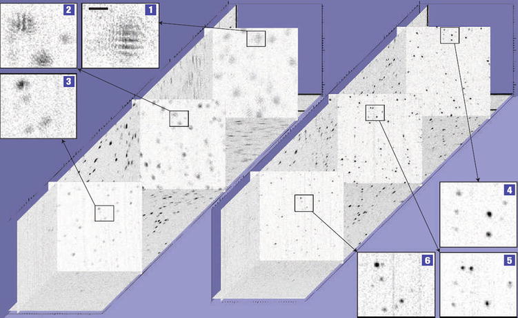
Fig. 31.2
Three-dimensional OCT (left) and ISAM (right) images of a silicone phantom containing titanium dioxide microparticles. The three en face planes in each dataset correspond to (1) z = 1,100 μm, (2) z = 475 μm, and (3) z = −240 μm, where z = 0 μm is the focal plane. The images were generated from a single 3D dataset acquired using an 800 nm SD-OCT system at an imaging NA of 0.05 (From [9])
31.3.2 Cross-Validation with OCT
It is obvious from Sect. 31.3.1 that ISAM provides significant improvements in resolution in the far-from-focus regime. But does three-dimensional ISAM accurately reconstruct the object structure? This question was addressed by comparing specific en face planes extracted from 3D ISAM reconstructions to in-focus OCT images of the same plane. In a sparse tissue phantom (see Fig. 31.3), the resolution and scatterer positions in an en face ISAM image are in excellent agreement to in-focus OCT of the same plane, demonstrating that ISAM provides an accurate reconstruction of the object. It should be noted that the signal-to-noise ratio (SNR) of the in-focus OCT is higher. This can be attributed to the increased light collection efficiency at the focal plane of the optical system, due to the 1/|z| depth dependence in the forward model describing the away-from-focus signal (see Eqs. 31.8 and 31.9). The improved signal collection at focus is the reason to place the object near the focus. In practice, the focus is positioned at approximately 50–75 % of the maximum imaging depth in a given sample.
Fig. 31.3
Cross-validation of ISAM and in-focus OCT in a silicone phantom containing titanium dioxide microparticles. (a) En face OCT from 3.75 Rayleigh ranges above the focus and (b) the same en face plane extracted from the 3D ISAM reconstruction. (c) In-focus OCT obtained by shifting the beam focus to the same depth as in (a) and (b). The inset in the lower left of each panel shows the relative depths of the displayed en face planes with respect to the beam focus. The two datasets were acquired using an 800 nm OCT system with an NA ∼ 0.05 (Adapted from [25])
For biomedical imaging applications it is important to confirm the reconstruction accuracy of ISAM in biological tissue. Figure 31.4 presents results of rat mammary tissue, once again comparing a specific en face plane extracted from 3D ISAM reconstructions to the in-focus OCT image of the same plane. Close agreement between structural features of tissue is seen between the far-from-focus ISAM reconstruction and the in-focus OCT. As with the phantom results, the in-focus OCT demonstrates higher SNR, resulting in better definition of structural features with weak signals. Additionally, since the acquisition rate was relatively low (0.6 frames/s), uncorrected phase instabilities may also result in degraded definition of weak signals. Sections 31.6 and 31.7 discuss the relevant data acquisition requirements, limitations of ISAM, and practical methods to address these limitations.
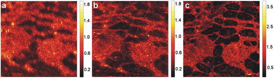
Fig. 31.4
Cross-validation of ISAM and in-focus OCT in rat mammary tissue. (a) En face OCT from eight Rayleigh ranges above the focus and (b) the same en face plane extracted from the 3D ISAM reconstruction. (c) In-focus OCT obtained by shifting the beam focus to the same depth as in (a) and (b). The datasets were acquired using an 800 nm OCT system with NA ∼ 0.1 (From [25])
31.3.3 Validation of ISAM with Histology
Histological analysis is the gold standard for diagnosing the pathological status of tissue. Thus, in order to test the accuracy of reconstruction in tissue, ISAM of resected human breast tissue was performed and compared to histology. Imaging was performed using an OCT system with 800 nm central wavelength and 100 nm bandwidth, with a focused beam numerical aperture of 0.05. Figure 31.5 shows a volumetric ISAM rendering and selected en face sections from near- and far-from-focus regions. The en face ISAM sections clearly provide improved resolution compared to OCT, over an extended depth-of-field. Tissue structure reconstructed by ISAM shows a close correspondence to histology, demonstrating that ISAM provides anatomically accurate reconstructions of biological tissue. This suggests that ISAM could be applied for high-resolution “optical biopsy” over a large imaging depth, as compared to OCM.
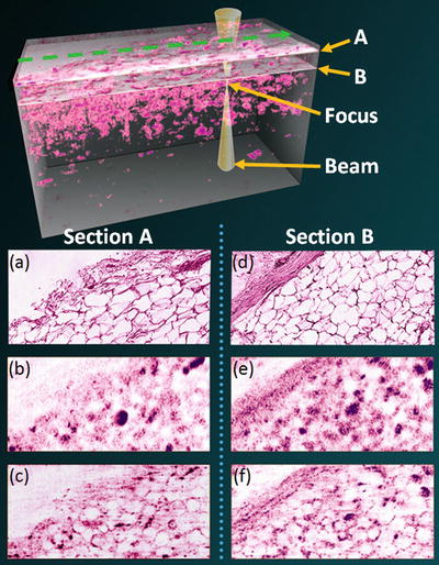
Fig. 31.5
Three-dimensional ISAM of resected human breast tissue compared with histology. En face images are shown for depths located at 643 μm (Section A) and 591 μm (Section B) above the focal plane. (a, d) Histological sections show comparable features with respect to the (b, e) OCT data and (c, f) the ISAM reconstructions. The ISAM reconstructions resolve features in the tissue which are not decipherable from the OCT data. To acquire this 3D dataset, the beam was raster scanned in the geometry shown at the top (dashed green arrow) (Adapted from [9])
31.4 Computational Adaptive Optics
31.4.1 Aberrated Forward Model
The forward model in Eq. 31.9, which forms the basis of ISAM, is essentially space invariant. Apart from a gradual depth-dependent amplitude variation (the main contribution being the 1/z signal decay with distance from focus), and a gradual through-focus variation of the (Gouy) phase, the transfer function of the instrument, H(Q x , Q y ; k),5 is space invariant. Spatially invariant resolution has been clearly demonstrated for ISAM reconstructions of data acquired with (near ideal) Gaussian beams [9, 15, 16, 25]. However, for an aberrated Gaussian beam, the ISAM reconstruction can produce a spatially varying point spread function, as seen, for example, by the asymmetry about the focus that is introduced by spherical aberration [13].
The effect of aberrations can be incorporated through a generalization of the forward model in Eq. 31.9. This approach considers the impact of aberrations as an extra (space-variant) filtering step in the forward model. In the general case, the effect of aberrations can have a dependence on all three spatial coordinates. This coupling between the space and frequency domains leads to an aberrated forward model that is defined in a piecewise manner over the spatial domain. This three-dimensional space-dependent imaging operation was considered by Frieden, who introduced the concept of an isotome [26], or volume of stationarity V(x 0, y 0, z 0) centered at position (x 0, y 0, z 0). The term isotome is a generalization of the term isoplanatic patch used in astronomical adaptive optics to denote the angular range over which a wavefront correction with hardware-based adaptive optics is valid [27]. The isotomic volume is then the region of space over which the 3D imaging operation can be considered space invariant. When restricted to one such isotome, the aberrated forward model can be written as

where H A (Q x , Q y , x, y, z; k) represents the extra (space-dependent) filtering step and  is the axial Fourier transform of the modified scattering potential defined in Eq. 31.8. In the general case, a different forward model of the signal may be required to describe the signal at different spatial locations.
(31.16)
is the axial Fourier transform of the modified scattering potential defined in Eq. 31.8. In the general case, a different forward model of the signal may be required to describe the signal at different spatial locations.In practice, space invariance in the transverse dimension is achieved over a relatively wide field of view, and Eq. 31.16 can be written for a slab volume geometry, V(z 0), centered at depth z 0 as

(31.17)
For the special case when the effects of particular aberrations are space invariant, V(x 0, y 0, z 0) is equal to the complete volume acquired, and Eq. 31.16 reduces to

where H A (Q x , Q y ; k) is an additional filtering step in the ISAM forward model of Eq. 31.9. When imaging with an ideal Gaussian beam, the instrument transfer function, H(Q x , Q y ; k), is slowly varying and can be ignored in practice. However, the phase distortions that aberrations induce across the bandwidth of the signal cannot be ignored since they can result in severe broadening of the point spread function or modify its functional form (i.e., to exhibit non-Gaussian structure).
(31.18)
31.4.2 The Computed Pupil and Hardware-Based AO
Computational adaptive optics is based on the Fourier optics result connecting the objective lens pupil function that is physically modified by hardware-based AO systems to the Fourier transform of the complex optical field at the nominal (aberration-free) focus. The objective lens pupil function, P(x, y), describes the deviation of the aberrated optical wavefront from an ideal spherical wavefront. It is related to the focal-plane transverse frequency response of the illumination beam according to [18]
where z f is the (object-side) focal length of the objective lens and the coordinate change (x, y) = (−2πz f Q x /k, − 2πz f Q y /k) provides the mapping between transverse spatial frequency and the spatial coordinates of the objective lens pupil. As done in Ref. [18], a prefactor of 2πAz f /k in the right-hand side of Eq. 31.19 has been set to unity. The pupil phase aberration, Φg, is included in the generalized pupil function [18]
![$$ P\left(x,y\right)={P}_{\mathrm{ideal}}\left(x,y\right) \exp \left[ik{\Phi}_{\mathrm{g}}\left(x,y\right)\right], $$](/wp-content/uploads/2017/03/A76297_2_En_32_Chapter_Equ20.gif)
where P ideal(x, y) for a typical OCT system is a real Gaussian envelope. Since the ideal beam focus is the impulse response of the (single-pass) imaging system,  can be regarded as the (transverse) amplitude transfer function [18]. Making use of Eqs. 31.4 and 31.19, the transverse Fourier domain of the aberrated OCT PSF may be written in terms of the objective lens pupil function as
![$$ \tilde{g}\left({Q}_x,{Q}_y,z;k\right)=i2\pi P\left(\frac{-2\pi {z}_f{Q}_x}{k},\frac{-2\pi {z}_f{Q}_y}{k}\right) \exp \left[i{k}_z\left({Q}_x,{Q}_y\right)z\right], $$](/wp-content/uploads/2017/03/A76297_2_En_32_Chapter_Equ21.gif)
where the phase of the pupil function, Φg (x, y), can conveniently be expressed as a sum of Zernike polynomials [14, 28], as is commonly done to represent aberrations in optical systems.6
(31.19)
(31.20)
can be regarded as the (transverse) amplitude transfer function [18]. Making use of Eqs. 31.4 and 31.19, the transverse Fourier domain of the aberrated OCT PSF may be written in terms of the objective lens pupil function as(31.21)
Due to the double-pass (epi-illumination) imaging geometry, the OCT PSF is related to the square of the optical beam [15, 16]. A computed pupil is defined here as the convolution of the pupil functions (see Eq. 31.5) that are physical modified by hardware-based AO. Note that this definition of the computed pupil uses the exact expression for the PSF, i.e., before the asymptotic approximations made by ISAM. This is important since the convolution operation (of phase-only pupil functions) can produce depth-dependent amplitude and phase structure in the transverse Fourier domain that is not preserved after the asymptotic approximations, such as that far-from-focus approximation in Eq. 31.6. In particular, depth-dependent amplitude structure in the transverse Fourier domain of the PSF,  , was found to contribute to the asymmetry about the beam focus when imaging with a beam that has spherical aberration [13].
, was found to contribute to the asymmetry about the beam focus when imaging with a beam that has spherical aberration [13].Aberrations of the computed pupil are described by an aberration filter, H A (Q x , Q y ; k), which are calculated as the deviation of the computed pupil function from its ideal functional form:
![$$ \begin{array}{l}{H}_A\left({Q}_x,{Q}_y,{z}_0;k\right)=\frac{{\tilde{h}}_A\left({Q}_x,{Q}_y,{z}_0;k\right){\tilde{h}}^{*}\left({Q}_x,{Q}_y,{z}_0;k\right)}{{\left|\tilde{h}\left(\operatorname{}{Q}_x,\operatorname{}{Q}_y,{z}_0;k\right)\right|}^2+\alpha}\\ {}=\frac{\left[{\tilde{g}}_A\left({Q}_x,{Q}_y,{z}_0;k\right){\otimes}_{\parallel }{\tilde{g}}_A\left({Q}_x,{Q}_y,{z}_0;k\right)\right]{\left[\tilde{g}\left({Q}_x,{Q}_y,{z}_0;k\right){\otimes}_{\parallel}\tilde{g}\left({Q}_x,{Q}_y,{z}_0;k\right)\right]}^{*}}{{\left|\tilde{g}\left({Q}_x,{Q}_y,{z}_0;k\right){\otimes}_{\parallel}\tilde{g}\left({Q}_x,{Q}_y,{z}_0;k\right)\right|}^2+\alpha },\end{array} $$](/wp-content/uploads/2017/03/A76297_2_En_32_Chapter_Equ22.gif)


