Quantitative Measurement of the Optic Disc and Retinal Nerve Fiber Layer
Kouros Nouri-Mahdavi
Joseph Caprioli
Glaucoma is an optic neuropathy characterized by a typical pattern of visual field loss and optic nerve damage as a result of retinal ganglion cell death. Alteration in the clinical appearance of the optic nerve head (ONH) and retinal nerve fiber layer (RNFL) frequently precedes the development of reproducible glaucomatous visual field defects1,2,3,4,5 In some patients with glaucoma, standard achromatic automated perimetry does not detect visual field defects until approximately 30% to 50% of retinal ganglion cell axons have been lost.6 Identification of structural changes is, therefore, important for the timely diagnosis and treatment of glaucoma and for monitoring its clinical course.
Until recently, assessment of the ONH and RNFL has been largely subjective. Variability in the size and appearance of the ONH and the number of ONH nerve fibers in normal eyes accounts for much of the difficulty in detecting the presence of early glaucomatous optic nerve damage. Standard techniques for diagnosis and monitoring structural change in glaucoma have included serial stereoscopic photographs of the optic disc and monochromatic photographs of the RNFL. While these methods provide objective information for sequential comparisons, the interpretation of the photographs remains subjective, and variation in photograph assessment among experienced observers is substantial.7,8,9 Similarly, expert observers’ agreement for detection of longitudinal change has been reported to be fair to good.10,11 However, qualitative longitudinal assessment of ONH stereo photographs may not be sufficiently sensitive to detect subtle changes in appearance over time. Also, knowing the chronologic order of change has been shown to significantly affect the reviewers’ opinions and their agreement among themselves.12
Many of the early innovative methods developed for quantitative analysis of the ONH and RNFL were not clinically practical. Planimetry has been used to quantify structural characteristics of the optic nerve head and peripapillary retina,13 but its subjectivity and poor reproducibility limited the ability of such measurements to recognize early glaucomatous damage. Stereophotogrammetry has been used to make subjective measurements from disc photographs, but is labor intensive and requires specialized stereoscopic plotting equipment and a highly skilled operator.14 With the development of new imaging technologies, instruments have become available to produce objective, accurate, and reproducible quantitative measurements of ONH and RNFL topography. In this chapter, we will review the basic principles and clinical application of several commercially available quantitative imaging methods: confocal scanning laser ophthalmoscopy, scanning laser polarimetry, and optical coherence tomography.
CONFOCAL SCANNING LASER OPHTHALMOSCOPY
Confocal scanning laser ophthalmoscopy (CSLO) provides real-time three-dimensional images of optic nerve topography. The only commercially available CSLO on the market is the Heidelberg Retina Tomograph (HRT, Heidelberg Engineering, Heidelberg, Germany). A 670-nm diode laser light source is used to scan the fundus in two dimensions. In a confocal scanning laser system, as shown in Figure 48A-1, scanners and scanning optics are used for both illumination and detection. The illuminating laser beam passes through a pinhole. A second pinhole, in front of the detector in a plane optically conjugate to the focal plane of the retina, acts as a filter. This allows only light reflected from the object at the focal plane to pass through the pinhole and be detected. Out-of-focus light reflections and scattered light are not focused on the detector and are suppressed. The reflected light at the detector is collected and measured in an array of pixels, creating a two-dimensional optical section of the retina at that focal plane.
 Figure 48A-1. Diagram of a confocal scanning laser system. The laser beam passes through a pinhole that sharply focuses the laser light at a focal plane on the optic disc. A second pinhole, in front of the detector, acts as a filter for the light emanating from the eye. This allows only light reflected from objects at the focal plane to be detected. |
A sequence of two-dimensional confocal optical section images can be recorded by changing the location of the focal plane along the optical axis, progressing from anterior to the ONH, through the ONH and ending posterior to the lamina cribrosa. A tomographic series typically consists of 16 to 64 sequentially scanned optical section images, allowing the object to be resolved spatially in three dimensions. The scan depth may range from 1 to 4 mm and is set by the machine. The imaging is repeated twice, and a mean topography image is produced from averaging the three sets of three-dimensional images. With the current version of HRT software (HRT 3), the field of view is fixed at 15 × 15°, and digitization is performed in frames of 384×384 pixels with a spatial resolution of 10 μm per pixel. The effective axial resolution (a function of the distance between sequential tomographic planes) is about 50 to 60 μm. Image acquisition takes approximately 1 to 2 seconds. The software stacks the series of tomographic images so that corresponding points on the retina are aligned horizontally and vertically to compensate for eye movement during image acquisition (Fig. 48A-2).
 Figure 48A-2. Confocal optical section images. The series of 32 images are stacked on top of each other so that corresponding points on the retina are aligned. |
To evaluate the topographic information, a contour line is drawn by the examiner around the inner margin of the peripapillary scleral ring to define the disc margin (Fig. 48A-3). The HRT software then establishes a reference plane 50 μm posterior to the retinal surface at the edge of the disc on the papillomacular bundle, between 350° and 356°. The reference plane is established at this location because the fibers in the papillomacular bundle are thought to be least affected as glaucoma progresses, thereby providing a relatively stable reference plane. As displayed in Figure 48A-4, all structures below the reference plane are defined as belonging to the optic cup (red) and all structures above the reference plane and within the contour line are considered as part of the neural rim (green for nonsloping rim and blue for sloping rim). Other reference planes have been explored over the years.15 In the newer software, the examiner has the option of using a 320-μm reference plane, which is associated with more stable measurements.16 A peripheral circle centered on the image frame with an outer diameter of 94% and a width 3% of the image size serves as the reference ring. The retinal height in the papillomacular bundle is used as the reference for the 320-μm reference plane, which lies 320 μm below the retinal height at the level of the reference ring. The new HRT 3 software (version 3.1.2.0) has led to improved image alignment and a more stable, consistent peripheral reference ring.17 Any reference plane based on the retinal or optic disc surface can be potentially affected in glaucoma.18 A modified reference plane, the Moorfields reference plane, has been shown to improve rim area reproducibility compared with the standard reference plane although it performs similar to HRT’s 320-μm reference plane.19
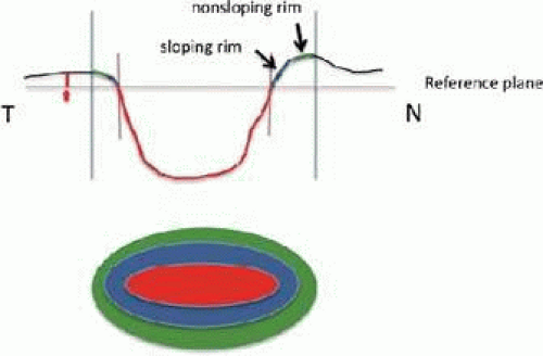 Figure 48A-3. Heidelberg Retina Tomograph (HRT; Heidelberg Engineering, Heidelberg, Germany) reference plane. The reference plane (red line) is defined as the plane located 50 microns below the retinal surface on the contour line at the temporal disc border between 350° and 356° (small red arrow). All structures below the reference plane are considered to belong to the optic cup (red), and all structures above the reference plane and within the contour line are considered to belong to neural rim (green for nonsloping rim and blue for sloping rim). The blue lines perpendicular to the reference plane represent the disc edge, and the red lines perpendicular to the reference plane represent the cup border. |
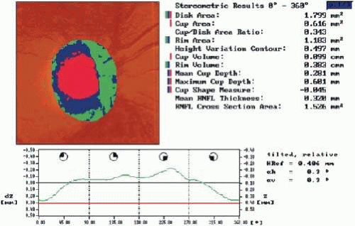 Figure 48A-4. Heidelberg Retina Tomograph (HRT; Heidelberg Engineering, Heidelberg, Germany) analysis: normal optic disc. The contour line height demonstrates a double hump pattern corresponding to the thicker distribution of nerve fibers along the superior and inferior poles of the optic nerve head. |
After the contour line is drawn, stereometric parameters of optic nerve head topography are generated, based on the division of the disc into rim and cup by the reference plane and include rim area, rim volume, cup area, cup volume, cup-to-disc ratio, mean RNFL thickness, RNFL cross-sectional area, mean and maximum cup depth, height variation contour, and cup shape measure. The height variation contour demonstrates the change of the retinal height along the contour line. Smaller height variation contour means flatter retinal height at superior and inferior poles and hence is evidence for possible glaucomatous damage. Cup shape measure is the statistical third moment of the distribution of all cup depth measurements. The third moment reflects departures from a symmetrical distribution around the mean and as such reflects the steepness of the rim slope. As expected, most of these parameters will change if the reference plane is modified.
In normal discs, the contour line height displays a double-hump pattern corresponding to the thicker distribution of nerve fibers along the superior and inferior poles of the ONH (Fig. 4). Glaucomatous structural damage is characterized by a reduction of parameters that describe rim structures (area, volume) and an increase in parameters that indicate tissue loss (more positive cup shape measure, increase in cup volume and cup-to-disc ratio). Glaucomatous alterations are typically associated with an asymmetrical or diffuse flattening of the contour line, or localized depressions corresponding to disc notches. An example of an HRT follow-up OU report along with the Glaucoma Probability Score report is shown in Figure 48A-5.
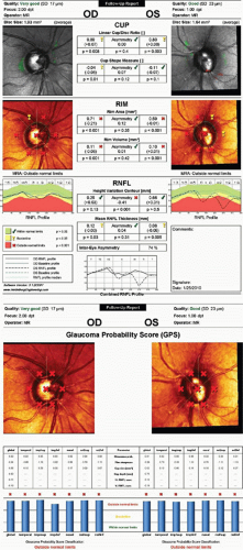 Figure 48A-5. Examples of the OU Follow-up report (A) and Glaucoma Probability Score (GPS) report (B) for the Heidelberg Retina Tomograph. A. The demographic characteristics of the patient have been deleted. On top, the quality of image, focus, and operator’s name are displayed for the right and left eyes. Below that, on the sides, the reflectance images with or without the contour lines are shown along with disc size in mm2 and a classification of disc size (small, average, large). In a follow-up exam, a summary of Topographic Change Analysis (TCA) results can be seen on top overlying a gray-scale version of the reflectance images. Green and red dots represent areas of statistically significantly increasing (improvement) and decreasing (worsening) pixel heights, respectively. No significant change is seen in either eye in this case. The black bands around the images represent areas of the image that have been trimmed by the image alignment algorithm since this is a follow-up report. Results of Moorfields Regression Analysis are schematically shown as checkmarks (within normal limits), exclamation marks (borderline) or Xs (outside normal limits) on the second row of reflectance images as well as in text. The graphs on the third row display retinal nerve fiber layer (RNFL) height along the contour line (RNFL profile). Green, yellow, and red bands represent regions of normal, borderline, and abnormal RNFL measurements, respectively. The black lines represent the patient’s actual RNFL profile compared to the baseline RNFL height (blue lines) while the green lines represent the median measurements for control subjects of the same age adjusted for disc size and ethnicity. In this example, significant loss of RNFL height inferotemporally on the left side can be observed, although the TCA fails to show any change. Six major stereometric parameters (linear cup/disc ratio, cup shape measure, rim area and volume, height variation contour, and mean retinal nerve fiber layer thickness) are displayed in the middle column, and results are compared between the two eyes (asymmetry) along with a p value for the asymmetry. An overall intereye asymmetry index is also provided below the RNFL parameters along with an overlay graph of the actual RNFL profiles of the two eyes. B. Again, the demographic characteristics of the patient have been deleted. Below, the quality of image, focus, and operator’s name are displayed for the right and left eyes. The GPS results are overlaid on reflectance images of both eyes. The interpretation of the symbols is the same as above. Lack of centration of the GPS symbols would reflect poor software performance, and results should therefore be ignored. The results are based on the global or sectoral glaucoma probabilities (whichever is worse) with numbers less than 0.28 considered normal, those greater than 0.64 considered glaucoma, and numbers in between flagged as borderline. The measurements for five main parameters from which the glaucoma probabilities are calculated are also provided (rim steepness, cup size, cup depth, and horizontal and vertical RNFL curvatures). |
The HRT software also provides a numeric score for quality of the image. The average variability (pixel standard deviation) among the three topographic images obtained in a single session is used to express the quality of the image. It can vary from less than 10 μm (excellent) to greater than 50 μm (poor).
Reproducibility
The reproducibility of a measurement is a prerequisite to determine the validity of a single measurement or to detect change in repeated measurements over time on the condition that measurements have high accuracy as well. With regard to optic nerve imaging, reproducibility is defined as the ability to obtain the same values in the absence of structural change. The magnitude of change that is detectable by the instrument is related to its reproducibility; the better the reproducibility, the smaller the change that can be detected. Test-retest variability must, therefore, be small to detect small but real interval progression of glaucomatous damage at the level of the ONH. Various investigators have reported high levels of reproducibility with CSLO.20,21,22,23 The reproducibility of height measurements has been shown to be between 10 and 20 μm, and the coefficients of variation of the stereometric parameters been reported to be approximately 5%. Mean standard deviation of test-retest variability was found to be significantly greater for glaucoma patients versus normal controls.24 Test-retest variability was also influenced by age, and was greater in older patients, likely a reflection of more frequent media opacity in this age group. Because glaucomatous discs tend to have a greater degree of sloping and excavation of the neural rim, and because the computer algorithm used to align the images has a higher error in areas of steep topographic slope, it is not surprising that glaucoma patients were found to have a higher degree of test-retest variability. No significant differences have been found between short-term and long-term variability estimates, indicating that measurements are not influenced by the time interval between measurements.25 Also, stereometric parameters have been shown not to significantly change with moderate intraocular pressure (IOP) variation.26
The new HRT3 Glaucoma Probability Score (GPS) software has shown good reproducibility in normal and glaucoma patients, with decreasing reproducibility with worsening image quality.27 Longitudinal reproducibility of HRT has been reported as acceptable and as such it compares well to other imaging devices.28
Accuracy
Histologic validation of measurements obtained with CSLO has been reported. Good correlation was found between in vivo optic disc topographic measures and histomorphometric measurements of optic nerve fiber number in primate eyes with laser-induced glaucoma.29 Plastic models have also been developed that have shown high levels of accuracy with CSLO.30 However, extrapolation of these results to a living human eye is difficult because of the different and complex optical properties of living human tissue.
Clinical correlation with CSLO measurements has concentrated on associations between topographic measures with visual function. A significant association between RNFL cross-sectional area and regional and hemifield measures of visual field loss has been reported.31 Peripapillary height,32 rim area, and cup shape measure33,34 have also been demonstrated to be highly correlated with global indices of visual function on achromatic perimetry. This association has also been confirmed with short-wavelength automated perimetry.35
Cup shape measure summarizes the structure of the cup and takes into account its depth variation and steepness of the cup walls, independent of both disc size and a retinal reference plane. This parameter is a good indicator of the severity of disc damage and appears to have the strongest relationship with visual field loss.36
Detection of Glaucoma, Sensitivity, and Specificity
Because of the large interindividual variability of normal optic nerve head topography, there is no technique, qualitative or quantitative, that will provide perfect discrimination between normal and glaucomatous eyes. It is therefore not surprising that there is considerable overlap in individual optic disc parameter measurements between healthy eyes and eyes with early to moderate glaucoma. Currently, HRT uses software with various statistical analyses to improve the discriminating ability between normal and glaucomatous eyes. These techniques include multivariate discriminant analyses, Moorfields Regression Analysis (MRA), and Glaucoma Probability Score (GPS). It must be noted that the performance of HRT, or any imaging device for that matter, is highly dependent on how glaucoma is defined.37 This is likely a result of how sensitive and specific any field criterion is to detect early glaucomas.
It has been found by several investigators that cup shape measure, rim volume, and retinal height variation contour are the most important parameters to differentiate between normal and glaucomatous optic discs.38,39,40 The sensitivity and specificity of various parameters in different studies has ranged between 62% to 87% and 80% to 96%, respectively.39,41,42,43 This wide variability in discriminating ability may be explained in part by different sample sizes, definitions of glaucoma, and varying degrees of glaucomatous optic nerve damage. Similarly, the area under radius of curvature.[1] curves (AUC) has been used to measure and compare the performance of HRT parameters for detection of glaucoma. The AUCs for HRT parameters have varied from 0.84 to 0.91 in different studies.44,45,46 A linear combination of various significant parameters has been used to compute the different linear discriminant functions available on the HRT (FS Mikelberg, Burk, and R Bathija discriminant functions) for classification of optic discs as normal or glaucomatous.47 An independent comparison of these discriminant methods has shown that none are very sensitive or quite specific48 although they are among the best performing parameters. Large discs (area >2.10 mm2) tended to be classified with a higher sensitivity but lower specificity than small discs (area <1.73 mm2). It should be reemphasized that the characteristics of the study population markedly influence the discriminating ability of any technique involved in differentiating glaucomatous from healthy eyes.
The Moorfields Regression Analysis (MRA) uses the neuroretinal rim area adjusted for the optic disc area, age, and ethnicity to determine whether a disc is within or outside the normal reference limits derived from a normative database (Fig. 5). Approximately 67% of eyes with early glaucoma are classified as outside normal limits, and a further 20% are borderline.43 Abnormalities other than glaucoma, such as tilted discs, may cause measurements to fall outside the normal range.
HRT’s normative database has been recently updated with introduction of HRT 3 software. It now includes 733 eyes of European ancestry, 215 eyes of African origin, and 104 Indian eyes. This has resulted in an improved sensitivity of overall MRA classification (65.3% vs. 50%) in black individuals, although at the price of diminished specificity (from 98.6% to 90.3%).49 The lower specificity may result from differences in the ethnic origin of the black individuals in the study (New York) compared with those in the normative database (Alabama). In a study conducted in Alabama, however, a similar higher sensitivity and lower specificity was observed for MRA with the new ethnic-specific database.50
The Glaucoma Probability Score or GPS has been introduced as another diagnostic option on the HRT 3 software for discrimination of glaucomatous from normal eyes.51 It is based on the geometrical three-dimensional modeling of the optic disc/peripapillary surface and the cup both globally and in six sectors of the optic disc.52 No user intervention or drawing of contour line is necessary. The resulting parameters are then interpreted by a relevance vector machine, a type of machine learning classifier. The GPS software provides the clinician with a numerical index that describes the estimated probability of presence of glaucoma. It ranges from 0 (low probability of glaucoma) to 1 (high probability of glaucoma). Scores between 0.28 and 0.64 are considered borderline abnormal while a score less than 0.28 is considered normal and any score greater than 0.64 is presumed to represent glaucomatous damage. Sectors classified as borderline or outside normal limits are flagged with yellow exclamation marks or red crosses, respectively. GPS’s reproducibility has been reported to be substantial to excellent in glaucomatous eyes.27 The result of the GPS analysis is determined by the global index or the sector with the highest probability score. GPS’s performance has been reported to be as good as the Moorfields Regression Analysis for separating glaucomatous from normal eyes, although, overall, the GPS seems to be somewhat more sensitive and less specific compared with MRA.52,53,54,55,56 However, one study reported a similar performance of MRA versus GPS.57 Zangwill et al58 compared the performance of MRA and GPS taking into account the effect of disc size and glaucoma severity. They found higher positive likelihood ratios for MRA and lower negative likelihood ratios for GPS. If these results are confirmed, it is possible that clinicians should be interpreting the two algorithms according to likelihood of presence of glaucoma in a particular patient before doing the test. In other words, GPS may be better suited to rule out glaucoma whereas MRA may be more suitable for ruling in glaucoma.
A larger disc area and more advanced glaucoma have been shown to improve the accuracy of glaucoma detection.58,59,60,61 The influence of disc area on the range of stereometric parameters has been observed in an elderly population surveyed.62 Disc area has been found to be larger in glaucoma patients in some of the more recent studies.50,52,58 The performance of GPS suffers serious setbacks when the disc is too small or the contour of the disc does not follow the geometrical assumptions of the model.50 GPS and MRA have been found to perform similarly across the spectrum of glaucoma severity.61 Sector-based analyses for MRA, stereometric analysis, and GPS have been explored, but there is not enough evidence that sector-based analyses are superior to global analyses. although a trend for better performance was observed with sector-based analyses.63
The Tajimi Study is the only population-based study that has reported performance of three different diagnostic modalities of HRT 3 (FSM discriminant function, MRA, and GPS).64 The sensitivities for all the three modalities were found to be lower compared to clinic-based series whereas the specificities remained consistent with the latter. MRA had the lowest sensitivity and the highest positive predictive value and specificity. Larger disc size led to decreasing sensitivity for all the modalities whereas older age and more hyperopic refraction caused only GPS to perform less specifically. The positive predictive values, i.e., the proportion of patients who are correctly diagnosed by the test, were generally poor (12%–23%), whereas the negative predictive values, or the proportion of normal subjects who are identified correctly by the test, were quite satisfactory (96%–99%). However, HRT’s performance expectedly improves when subjects at higher-than-average risk for glaucoma are screened.65 Neural networks improve HRT’s performance,66 but there is no commercial software available yet that uses artificial intelligence for this purpose.
Ability to Detect Change over Time
As of now, there is no evidence that CSLO can improve our ability to detect progression of glaucoma as compared with qualitative evaluation of stereoscopic disc photographs. Because progression of glaucoma is slow, years of follow-up are needed to answer this question. Follow-up studies in monkeys67 and in patients after surgery68,69 or medical reduction of intraocular pressure70 have been used as surrogates to more rapidly determine which analysis strategies are best to identify clinically relevant progression of glaucoma.
Image quality is the main determinant of noise level and variability in cross-sectional and longitudinal series of HRT images.71 Rim area variability is reportedly highest in nasal and temporal segments of the optic rim. Estimation of rates of progression with HRT has confirmed that the inferotemporal and superotemporal regions of the neuroretinal rim demonstrate the highest frequency and rates of loss.72
Many different methods have been developed over the last decade for detection of progression with HRT. The longitudinal variability of HRT has been reported to be acceptable.28 Global and regional changes in stereometric optic disc parameters can be monitored over time. Similar to visual fields, two main techniques have been applied to stereometric parameters for detection of progression. The first one is trend analysis or a simple linear regression analysis of disc parameters such as rim area against time. Trend analysis strategies that are available on the current software normalize stereometric parameters for graphical presentation with values ranging from 0 to -1. Zero indicates the average measurements of a given stereometric parameter in normal subjects whereas -1 indicates maximal loss according to the same parameter in advanced glaucoma patients. The second technique, called event analysis, has been mostly applied to rim area and consists of comparing global and segmental rim area measurements from each follow-up exam to those of baseline images with change being flagged when the new measurements fall outside the limits of variability for baseline images.73 The advantage of event analyses is lack of need for numerous images before they reach a reasonable sensitivity, as compared to trend analyses. Also, the criteria for these types of analyses can be modified according to image variability.17 Using stringent criteria, event analysis of rim area has been shown to have very good specificity while detecting a larger proportion of progressing eyes compared to trend analyses. A newer technique of statistical image mapping has been recently introduced and seems to demonstrate good sensitivity and specificity compared to Topographic Change Analysis and trend analysis of the rim area.74
Topographic Change Analysis or TCA is based on the evaluation of arrays of condensed superpixels from individual topographic images for which location-specific confidence intervals have been determined. Simply put, the program compares changes in predefined superpixel heights over time. Superpixels consist of an array of 4×4 pixels within the HRT image.75 The average change in the superpixel height is corrected for the correlation of the 16 pixels inside the superpixel and the variability of baseline and follow-up images. The analysis includes a color-coded image of absolute and statistically significant change in superpixels over time. One of the main advantages of TCA is provision of location-specific change information. In addition, there is no need to outline the disc margin or to determine a reference plane. Figure 48A-6 demonstrates an example of significant progression as evidenced by rim loss inferiorly on optic disc photographs, TCA, and the trend analysis for rim area.
 Figure 48A-6. An example of optic disc progression detected by both disc photographs and HRT. A. Recurrent disc hemorrhages and slow progressive loss of the inferior disc rim can be observed. B. Starting in 2000, some loss of the neuroretinal rim is observed on HRT’s Topographic Change Analysis, although the change become more remarkable only in 2002. The nerve fiber layer wedge defect can also be seen on HRT images. C. The trend analysis for rim area demonstrates a consistent downward trend inferotemporally with the normalized rim area showing maximal loss (-1.0) by 2007. |
There are limited data in the literature with regard to longitudinal comparison of detection of change with HRT and performance of experienced observers for review of stereoscopic disc photographs.9,76,77,78,79,80 High rates of progression compared to performance of visual fields and qualitative evaluation of optic disc photographs have been reported although in that series good concordance (80% agreement) was seen with review of optic disc photographs in a small subgroup of patients.81 Chauhan et al9 recently investigated the performance of experienced observers to that of TCA for detection of disc progression. Overall agreement between observers was better than that of observers and TCA. The results, however, depended on the criteria used (conservative vs. less stringent). TCA performed as well as expert observers in this study. However, another study found poor correlation between HRT’s TCA, MRA, and trend analyses of stereometric parameters, and agreement of experienced observers, when progression was defined according to HRT’s software criteria.80 A recent study compared prevalence of prior disc change based on TCA in a group of glaucoma patients.82 Eyes progressing according to stringent field criteria were about three times more likely to have shown prior disc worsening. Various HRT parameters, including MRA and GPS, have been found to be predictive of future conversion to glaucoma in OHT or glaucoma suspect eyes.83,84,85
Advantages
CSLO provides objective, reproducible, quantitative assessment of the ONH. Three-dimensional topographic maps of the ONH can be obtained in approximately 1 second with real-time feedback to the operator with regard to quality of imaging in most cases. Images can be obtained even with moderate cataract and do not require pupillary dilation. Introduction of race-specific normative databases may lead to some improvement in performance of the machine. No mechanical storage is necessary, and multiple topographic summary parameters are obtainable with automated techniques. The newer generations of HRT are all backward compatible. Images obtained with previous versions of the device can be viewed and combined with images taken with the newer versions to detect progression although image alignment is not always perfect.
Disadvantages
The considerable variation in optic disc topography among normal eyes necessitates a large age- and race-specific normative database that has recently been established. Further studies are needed to determine whether this will lead to better performance of the device. Technological limitations include the use of a standard reference plane and the need for correct placement of the disc margin by the operator, both of which can influence many of the topographic indices generated. Assessment of optic disc topography is only one aspect of the clinical evaluation for glaucoma. Other features of glaucoma including RNFL damage, peripapillary atrophy, and disc hemorrhages can be missed by sole reliance on this technique for monitoring of glaucoma.
SCANNING LASER POLARIMETRY
Scanning laser polarimetry (SLP) is designed to quantitatively assess the thickness of the peripapillary RNFL. It is based on the measurement of a physical property called retardation of an illuminating laser beam passing through the birefringent RNFL. As depicted in Figure 48A-7, birefringence in the nerve fiber layer arises from the parallel arrangement of microtubules within the RNFL. This causes a change in the state of polarization of the light passing through the RNFL that is assumed to be linearly related to its thickness. Light polarized in one plane travels more slowly through the birefringent RNFL than light polarized perpendicularly to it. This difference in speed causes a phase shift (retardation) between the perpendicular light beams.
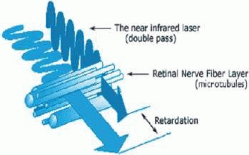 Figure 48A-7. Nerve fiber layer birefringence. Birefringence in the nerve fiber layer arises from the parallel arrangement of microtubules within the retinal nerve fiber layer (RNFL). Light polarized in one plane travels more slowly through the birefringent RNFL than light polarized perpendicularly to it. This difference in speed causes a phase shift (retardation) between the perpendicular light beams, which is proportional to the RNFL thickness. |
A 785-nm diode confocal scanning laser with an integrated polarimeter is focused on the retina. The backscattered light that doubly passes through the RNFL shows retardation that is linearly related to the RNFL thickness and is measured by a polarization detection unit. The total data acquisition takes 0.7 seconds. Two images of each eye are obtained, the first one to determine the anterior segment birefringence and the second one to measure adjusted retinal birefringence. Each image measures 20 × 20° and contains 16,384 (128×128) pixels. A reflectance image of the scanned image is produced. The software then outlines the optic disc margin using an ellipse that can be recentered manually. Retardation values are automatically generated along a 8-pixel-wide ring concentric with the disc with an outer diameter of 3.2 mm and inner diameter of 2.5 mm. The thickness values along the perimeter of the disc are then plotted as a cross-sectional graph.
The retardation pattern shows a pattern consistent with the RNFL thickness, and measurements seem to be stable and consistent at distances from the disc where the RNFL is usually measured.86 Areas of high retardation are displayed in yellow and white, and areas of low retardation displayed in blue. Figure 48A-8 shows an example of a healthy eye, demonstrating the typical double-hump curve, representing a cross-section of the two arcuate bundles, with the nasal, usually thinner, area in the center and the temporal area on the sides. Figure 48A-9 shows an example of glaucomatous damage with thinning of the RNFL in both superior and inferior arcuate areas. Retardation is markedly attenuated and the double-hump curve is significantly depressed, especially in the superotemporal quadrants.
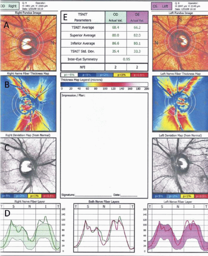 Figure 48A-8. An example of a normal SLP-VCC image from a 33-year-old male subject. On top, the eye, the Q-factor, and date are listed. Quality factor (Q) ranges from 1 to 10 with 10 representing the best quality. A Q factor >7 is considered acceptable. Topmost left or right; A. Reflectance images (right and left fundus images) represent a fundus-like picture, where potential issues with imaging such as decentration, poor focusing or illumination, movement during image acquisition, or floaters can be detected. The reflectance image should be uniformly illuminated. In presence of significant peripapillary atrophy, the measurement ring should be manually enlarged so that TSNIT parameters are calculated beyond the area of atrophy. B. Birefringence maps (right and left nerve fiber thickness maps): color-coded RNFL thickness measurements are shown with brighter, warmer colors representing thicker areas. The TSNIT parameters are calculated from measurements performed within the two rings surrounding the disc ellipse. C. The deviation maps demonstrate areas that are statistically significantly different from the normative database. A scale for statistical significance is also provided. Nasal areas sometimes show abnormalities that are likely not clinically significant. The NFL loss should be consistent with patterns of glaucomatous loss to be considered meaningful. D. TSNIT plots (right and left nerve fiber layers): the average NFL thickness within the TSNIT ring is plotted with bands of normality shown in green (right eye) or purple (left eye). The overlay plot in the middle can be used to compare RNFL symmetry in the two eyes. E. TSNIT parameters can be seen in the middle on top of the printout. Except for NFI (Nerve Fiber Indicator), all parameters are color-coded based on statistical significance. All parameters are based on the TSNIT measurement ring around the disc (2.5 mm internal diameter, 8 pixels in width). NFI deserves special attention since it is the best discriminating parameter for glaucoma in isolation. Values greater than 30 should be considered suspicious with values greater than 50 representing likely glaucoma. |
 Figure 48A-9. Example of a SLP-VCC report in a glaucomatous eye. Thinning of the superotemporal RNFL is seen bilaterally. Retardation is markedly attenuated, and the double-hump curve is significantly depressed in the superotemporal quadrants along with milder RNFL loss in inferotemporal regions. The deviation maps demonstrate defects in both superotemporal and inferotemporal areas bilaterally. The NFI is borderline OD while it is clearly above normal limits on the left side. Only the superior average on the left side is flagged as abnormal by the device in this particular case. |
A computer algorithm automatically generates retardation measurements throughout the peripapillary region and along the measurement ellipse. Average quadratic measurements, measurement ratios, symmetry measurements between superior and inferior quadrants, and modulation parameters are calculated. An index, called Nerve Fiber Indicator (NFI), is also generated and is the result of a linear vector support neural network that reflects the probability of glaucoma on a scale of 1 to 100. In most studies, the NFI has been the best parameter for discrimination of glaucoma from normal with values greater than 30 being considered borderline abnormal and values greater than 50 definitely abnormal.
Stay updated, free articles. Join our Telegram channel

Full access? Get Clinical Tree


