Corneal Topography and Wavefront Analysis: Optics and Clinical Applications
Yaron S. Rabinowitz
The anterior surface of the eye, with its tear film, is the major refractive element of the eye, and even minute disruptions of either component can result in decreased vision. These minor distortions in tear film or anterior corneal curvature are often not appreciated on slit-lamp examination and are best evaluated by methods that measure the topography of the cornea. Topography is the science of describing or representing the features of a particular surface.1 The most widely used technique to assess corneal shape employs the reflection of a target object from the anterior corneal surface with convex mirror optical principles.1 The ophthalmometer (Keratometer; Bausch and Lomb, Rochester, NY) is one such device. This device enables the radius of curvature of the anterior corneal surface to be determined from four reflected points approximately 3 mm apart. The Keratometer is limited by the fact that it provides no meaningful information regarding corneal shape central or peripheral to these points. Photokeratoscopes, which employ optical principles that are similar to those of the Keratometer, measure a larger surface area and provide a more complete appreciation of corneal shape.
The first known keratoscope target was the image of a window, as reported by Scheiner in 1619 using natural light. He estimated the corneal curvature by comparing the window pane corneal reflection to those of a series of marbles until he found one that gave an image the same size as that of the cornea.1 In 1820 Cuignet developed a keratoscope through which he observed the reflected image of an illuminated target held in front of a patient’s cornea. His major problem was in the alignment of the light, target, and observer with the patient’s visual axis. This was overcome in 1882 by Placido, who placed an observation hole in the center of the target.2 Placido’s target of alternating black and white rings (the Placido disk) has been embodied in many devices that are currently used to measure corneal topography, hence the term Placido disk keratoscopy.
A modern version of the original Placido disk is the Klein hand-held keratoscope (Fig. 65-1). This device is useful for detecting the location of tight sutures, irregular astigmatism, and keratoconus, all of which can be detected by mire pattern recognition. Its main limitations are that its mire pattern has an outer diameter of 5.5 mm, limiting its utility for evaluating peripheral topography. In addition there is no mechanism to achieve alignment other than user estimation, which introduces significant error in subjective interpretation.1 Photokeratoscopes (e.g., Corneascope; Keravision, Santa Clara, CA) project a series of concentric circular mires that form a virtual image located within the anterior chamber of the eye. Information regarding the power of the anterior corneal surfaces is derived from visual inspection of the size and shape of the mires.
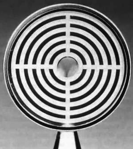 Fig. 65-1. Klein hand-held keratoscope. (From Rabinowitz YS, Wilson SE, Klyce SD (eds): A Color Atlas of Corneal Topography: Interpreting Videokeratography. Tokyo: Igaku Shoin Medical Publishers, 1993, with permission.) |
Simultaneously, information regarding the radius of curvature of a localized area of the cornea can be obtained by observing the separation between the mires reflected from that area of the cornea. In areas of steep cornea, the images of the mires are smaller, so the rings appear narrower and closer together. In the presence of regular astigmatism, the mires appear elliptic, the short axis of the ellipse corresponding to the meridian corneal steepening and highest power.3 Irregular astigmatism produces nonelliptic distortion of the mires. For the most part, photokeratoscopes yield qualitative information that is clinically useful as a means of evaluating changes in the peripheral cornea, such as in the detection of the corneal ectasia associated with keratoconus (Fig. 65-2), or as a guide to selective suture removal after penetrating keratoplasty. Its limitations are that it provides no information about the central 3 mm of the cornea and that up to 3 diopters of cylinder may go undetected by visual inspection of photokeratographs.
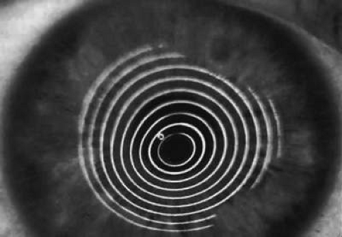 Fig. 65-2. Corneoscope keratograph depicting inferotemporal steepening in a patient with keratoconus. (From Rabinowitz YS, Wilson SE, Klyce SD (eds): A Color Atlas of Corneal Topography: Interpreting Videokeratography. Tokyo: Igaku Shoin Medical Publishers, 1993, with permission.) |
Quantitative analysis of photokeratograms became practical when Gullstrand in 1896 applied photography to keratoscopy (photokeratoscopy).3 This allowed the clinician to fix the image and measure the size of the rings; however, this analysis is slow and subject to major errors.3 In the 1980s, computer power was adapted to the task of automated high-resolution corneal topography analysis, which is most popularly implemented in commercially available computer-assisted videokeratoscopes, such as the Topographic Modeling System (TMS-1) (Computed Anatomy, New York, NY) and the Corneal Analysis System (Eysys Laboratories, Houston, TX). These devices were devised in order to overcome the deficiencies of photokeratoscopes both in speed and in gathering quantitative information about the anterior corneal surface.4 Most systems use illuminated Placido-type mires with nosecones that provide a broad area of corneal coverage from the apex to the limbus of the cornea, covering approximately 11 mm of cornea (Fig. 65-3). These novel conical mire targets provide very high radial resolution, being approximately 0.17 mm apart reflected on the normal corneal surface. Additionally, the central fixation light and the first mire of the standard cone provide excellent central corneal coverage, ensuring that corneal topographic details important to visual function are not obscured as they are with keratometers and traditional keratoscopic targets. Because direct measurements are made from the centrally visually important area as well as from the periphery, a clinically complete data set derived from between 6,000 and 11,000 data points on the cornea is available for clinical interpretation. Other advantages of videokeratoscopy over photokeratoscopy are its speed in gathering quantitative information and its ability to display data in a clinically useful format with reasonable accuracy.5,6,7
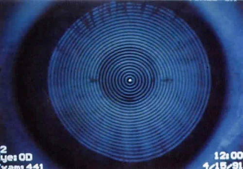 Fig. 65-3. Placido-disk reflection of videokeratoscope showing 32 rings. |
COMPUTER-ASSISTED VIDEOKERATOSCOPY
Computer-assisted videokeratoscopes consist of a Placido disk, a slit-lamp chin rest, and a video camera hooked up to a computer. In the Topographic Modeling System, the patient places his or her chin on a chin rest and is asked to look at a fixation target in the nosecone of the system (Figs. 65-4 and 65-5). The operator, who can view the Placido-disc mires on the video, brings them into focus with a joy stick and tries to bring a central target to the center of the pupil. Two peripheral targets also aid in focusing.
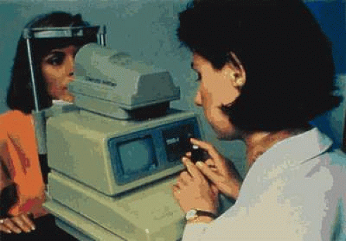 Fig. 65-4. Topographic Modeling System showing videocapturing of a patient’s anterior corneal surface. |
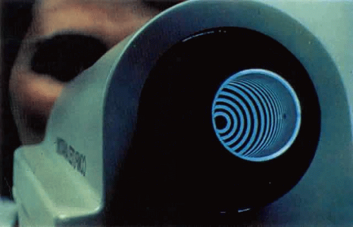 Fig. 65-5. Nosecone of the Topographic Modeling System videokeratoscope. |
When the three targets overlap, maximum focus has been reached and an electronic snapshot of the video picture of the reflection of the Placido mires is taken. The computer analyzes the image to determine the size and shape of the mires; it reconstructs the patient’s corneal surface and presents a graphic picture of the patient’s topography in a suitable form.
The most useful form of data presentation is a color-coded corneal contour map in which steep areas are depicted as warm colors, such as reds and browns, and shallow areas as cool colors, such as blues and greens (Fig. 65-6). Two scales are commonly used: absolute and normalized. In the absolute scale, each color represents a 1.5-diopter interval between 35 and 50 diopters, whereas above and below this range, colors represent 5-diopter intervals. This scale is useful in routine practice (e.g., preoperative screening). In the normalized scale, the cornea is divided into 11 equal colors spanning that eye’s total dioptric power. In this scale, more minute topographic details within an individual cornea are appreciated.8,9 An isometric plot is also available in which the cornea is viewed side on, allowing the observer to appreciate the relative depth of a corneal incision. As part of the topographic display, quantitative indices are also generated, including the following: predicted visual acuity based on corneal shape, simulated keratometry readings, minimum keratometry reading, surface regularity index, and surface asymmetry index.10
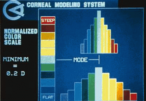 Fig. 65-6. Color scale used in videokeratographs. |
OPTICS
Calculation of Corneal Surface Power
Videokeratoscopic analysis of corneal shape relies on the optical principal that the tear film on the anterior corneal surface acts as a convex mirror. A light (mire) shined toward the cornea gives rise to a virtually erect image located approximately 4 mm posterior to the anterior surface of the cornea, at the level of the anterior lens capsule. This is the corneal light reflex, or first Purkinje-Sanson image, which is viewed during both keratoscopy and keratometry. The size of this image can be used to quantify the curvature of the cornea: the steeper the cornea (i.e., the smaller the radius of curvature), the more powerful the convex mirror is, and the smaller the image will be. By the same principles, any toricity (different radii of curvature in different meridians) or irregularity of the corneal surface will cause a regular or irregular distortion of the image.2 The image formed by a convex mirror can be constructed using two rays: (i) a ray parallel to the principal axis, which is reflected away from the principal focus; and (ii) a ray from the top of the object traveling toward the center of curvature and reflecting back along the same path (Fig. 65-7). The magnification produced by a curved mirror is the ratio of the image size (I) to the object size (O); this, in turn, is proportional to the ratio of the distances of the image (v) and the object (u) from the mirror, as follows:
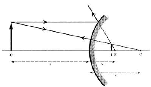 Fig. 65-7. Ray diagram depicting ray tracing in convex mirrors. (From Corbett MC, O’Bart DPS, Saunders DC, et al. The assessment of corneal topography. Eur J Implant Refract Surg 1994;6:98, with permission.) |
Magnification = I/O = v/u
In practice, the image (I) is located very close to the focal point (F), which is halfway between the center of curvature of the mirror (C, at the principal focus) and the mirror itself. Therefore v may be taken to equal half the radius of curvature of the mirror (r/2). Upon substituting r/2 for v in the preceding equation (I = O × r/2u), it can be seen that as the cornea becomes steeper and its radius of curvature (r) becomes smaller, so the image (I) also becomes smaller, and the topography mires appear closer together.
In a given keratometer, u is constant, being the focal distance of the viewing telescope. Rearrangement of the equation (r = 2u × I/O) shows that the radius of curvature is proportional to the image size if the object size remains constant.2 The geometric optics equation that relates corneal power in diopters (D) to the radius of corneal curvature (Rc, measured in millimeters) is adapted from Snell’s law of refraction, with differences of refractive index combined with corneal thickness and corneal back surface power to give the following equation:
D = Ki/Rc
where Ki is the keratometric index usually assigned a numeric value of 337.5. For example, a cornea with a radius of curvature (Rc) of 7.8 mm equates with this convention to a corneal power of 43.25 diopters (i.e., 337.5/7.8). The keratometric index differs from the corneal refractive index (1.376) in that it takes into account both the anterior and posterior corneal surfaces; however, it fails to recognize the differing refractive properties of the epithelium and the stroma.1
Corneal Contour Display
The corneal contour is usually described in one of three ways: qualitative, mathematic, or point-to-point. In the qualitative method, the cornea is said to consist of two zones: a central zone or corneal cap of nearly constant curvature, surrounded by a peripheral zone with an increasingly longer radius of curvature. The corneal cap is an artifact of measurement methods and continues to be used only because it provides a convenient clinical construct. The cornea actually has a radius of curvature that begins to change immediately as one moves away from the apex. Near the apex, the rate of change is slow but increases rapidly toward the periphery. Therefore, the cap diameter depends on an arbitrary criterion for the amount of radius change that can occur before it is considered significant: 1 diopter of change has typically been adopted as a criterion, which yields a corneal cap of approximately 4 mm.11,12
The second method of describing corneal contour is the mathematic method, which uses expressions such as an ellipse or polynomial. This method is favored by most because it has a number of applications to the optics of the eye, such as the analysis of aberrations. Of the various simple mathematic expressions that can be used to describe the cornea, the ellipse is the best. It is usually possible to align an elliptic curve very closely with radius data from any single meridian or hemimeridian of the cornea. It is only at the corneal periphery that the rate of flattening exceeds that of an ellipse. Thus, for the optic portion of the cornea, the ellipse is an adequate model.2,11
The third approach is the point-to-point method, which simply consists of an array of corneal radius or power values found at various corneal positions. Although this method seems simple and straightforward, it is difficult to assimilate an overall impression of the corneal contour merely by looking at an array of numbers; however, if all adjacent numbers with the same values are connected, as in contour mapping, the display is transformed into a comprehensible pattern that provides an overall impression of the corneal shape. Currently, the preferred method of displaying the corneal topography by videokeratoscopy is the topographic map. This method provides a large amount of information about the corneal contour in a single display. The corneal topographic map applies the principles of a geographic topographic map, except that instead of representing equal elevations, the isometric zones represent equal radii of curvature. The topographic map is derived from the radius measurements at several thousand corneal positions, which can be displayed either in millimeters of curvature or in dioptric power values. The diopters that are used for corneal power, however, have only a relative relationship to the true corneal power in the optical sense. For example if a cornea has a power of 42 diopters at the apex and 40 diopters at some peripheral point, we would expect the peripheral point to be 2 diopters out of focus. With current videokeratoscopy, however, the radius of curvature is actually measured, and the power displayed simply represents a conversion from radius to power using the following keratometric formula:
P = (n – 1)/r
where n equals 1.3375. This formula is not applicable to the peripheral cornea because the keratometric formula is valid only for paraxial rays and becomes increasingly inaccurate as one moves further peripherally. The power used in the calculation of the corneal topographic map is based on the keratometric formula and uses the radius of curvature (AC) ending at the optic axis (Fig. 65-8).11
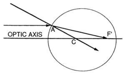 Fig. 65-8. Ray diagram illustrating radius of curvature AC used in the corneal power calculation of topographic maps. (From Mandell RB. The enigma of corneal contour. CLAO J 1992;18:267, with permission.) |
Alignment
Currently videokeratoscopes are aligned along an axis that is neither the line of sight nor the visual axis, both of which could be practical reference points. The subject looks at a fixation point on the optic axis of the instrument. The videokeratoscopic axis is aligned perpendicular to the cornea and thus is directed toward the center of curvature of the cornea for some unknown peripheral position (Fig. 65-9).11
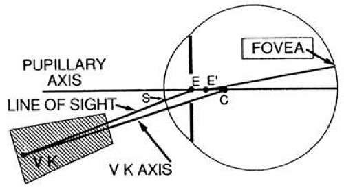 Fig. 65-9. Diagram showing alignment of videokeratoscope axis relative to the cornea, pupillary axis, and line of sight. (From Mandell RB: The enigma of corneal contour. CLAO J 1992;18:267, with permission.) |
Image Processing
From an optical standpoint the videokeratoscope has no advantage over the photokeratoscope; however, it is superior to the photokeratoscope in terms of image processing. What used to require hours or even days to analyze by hand can now be done in a few minutes. Not only are the measurements faster, they are more accurate. For example with manual digitization, a resolution of 500 lines/frame gives an accuracy of 1.2 diopters; automated digitization statistical procedures can achieve subpixel resolution and an accuracy of less than 0.25 diopters. Formerly it required great skill to construct a photokeratoscope with target rings that were perfectly round so that object size would be the same in all meridians. With the videokeratoscope, the target roundness is immaterial because every meridian can be calibrated separately. The ability of the instrument to measure the curvature of any small area depends largely on the instrument algorithm, which is a series of calculations involved in converting the videokeratoscope image sizes into radius of curvature values for the cornea.2
Software
A reference point is established from which the position of each point can be identified mathematically. Ideally the reference point should be related to an ocular feature such as the visual axis or corneal apex, but because the area of the cornea forming the sharpest retinal image is frequently not centered on any of these landmarks, it is often more appropriate to select the most convenient reproducible reference point. Most systems use the center of the innermost mire, the position of which can be determined in three ways. If the first mire is relatively large, computational techniques must be used to calculate either the centroid of its corneal surface area or its geometrically averaged center. These techniques have been obviated since the development of collimated devices, which can reduce the diameter of the innermost mire to 0.7 mm and use the reflection of the fixation light as the central reference point. The accuracy of the reference center depends on patient fixation and proper alignment of the instrument. Once a central reference point is established, rectangular coordinates are given to each data point where a semimeridian intersects a mire. Most commercial systems have 15 to 38 circular mires and 256 to 360 equally spaced semimeridians, theoretically providing between 6,000 and 11,000 data points.
The accuracy of the final reconstruction does not depend on the total number of data points, but on their density as long as the same video pixel is not sampled multiple times.2 The rectangular coordinates locating the data points are converted to polar coordinates on the keratoscope mires to facilitate corneal reconstruction. A reconstruction algorithm is then applied to the location of each point on the two-dimensional reflection to give the three-dimensional position of the cornea from which that reflection originated. The algorithm consists of a mathematic formula from which the curvature of the anterior corneal surface is calculated. This is then converted to total corneal power by the standard keratometric index.2 Because there is no known mathematic formula that describes the shape of the normal cornea, the algorithm gives only an approximation of corneal shape, which is most accurate centrally, where the cornea is most spheric. For each point on mire reflection to correspond to a unique position for the cornea, the following assumptions about the cornea are made: the surface is spheric within the small area being measured, the surface is of uniform refractive index, and the centers of curvature for all reflecting points are on the optic axis. Algorithms are derived in several ways. In the one-step curve-fitting method, the geometry of the reflected mires is globally fitted to a polynomial. A refinement fits the global geometric model to the cornea at each meridian individually, with allowance for local nonconformance. The one-step profile method normalizes the central radius of curvature to a standard 7.8 mm and then uses a successive approximation method to calculate the corneal shape in the periphery in a given meridian.
Stay updated, free articles. Join our Telegram channel

Full access? Get Clinical Tree


