Basic Statistics and Epidemiology for Ophthalmologists
Andrew F. Smith
The focus of this chapter is to explore and explain the main mathematic concepts used to describe and interpret the complex range of biologic, environmental, and other factors that impact on ocular morbidity (disease) and mortality (death). At a minimum, this chapter increases the ophthalmologist’s level of understanding of statistical and epidemiologic concepts and terminology used in the design, analysis, and interpretation of ophthalmic studies and data. At a maximum, this increased knowledge should result in the development of new, more efficacious, cost-effective, and evidence-based treatments and interventions that promote healthy eyesight, the prevention of vision loss, and, where possible, the reversal of blindness. The material is presented in short, discreet sections beginning with the fundamental concepts and proceeding to more advanced concepts.
POPULATION AND SAMPLES
A fundamental principle of statistics resides in being able to draw conclusions about a given population from a representative sample selected at random. In this respect, populations can either be finite, such as the number of operating theaters available at any one time, or infinite in the sense that one can sum all the possible outcomes arising from successive tosses of a coin, be it heads or tails.
INDUCTIVE VERSUS DEDUCTIVE STATISTICS
Theoretically, statistics can be divided into two broad camps, namely, inductive and deductive statistics. Inductive or inferential statistics relies on the use of probabilities to measure the potential that a given event will or will not take place. By contrast, deductive or descriptive statistics presents the data as they are rather than drawing conclusions from them.
TYPES OF VARIABLES
A variable may be thought of as a letter or symbol that can take on a predetermined set of values, which are denoted by the domain of a variable. Thus, a constant is a variable for which there is only one value. Continuous variables can assume any value between two other given values, such as 0 to 1, or 90 to 100, and all values in between. A discreet variable, by contrast, can move only from one value to the next in accordance with a set pattern. In addition, four broad types of variables can be defined. Nominal and ordinal variables refer to specific categories and require the use of “nonparametric” statistics to analyze them. By contrast, interval and ratio variables provide actual measurements and, as such, require the use of “parametric” statistical methods to be analyzed (Table 1).
TABLE 1. Types of Variables | ||||||||||||||||||
|---|---|---|---|---|---|---|---|---|---|---|---|---|---|---|---|---|---|---|
|
FREQUENCY DISTRIBUTIONS
To organize raw data into a more meaningful format, statisticians often sort data into various classes or categories. The number of cases within a particular class is called the class frequency, and the arrangement of all of the classes or categories into a table format yields the frequency distribution for that particular set of data. In Table 2, for example, 30 patients have been grouped according to their intraocular pressure readings into seven categories. The resulting distribution of the number of patients in each of the intraocular pressure categories is called a frequency distribution. The relative frequency distribution for the same group of patients can be found by adding up all of the patients in each intraocular pressure category and dividing by the total number of patients examined, in this case, 30. Often, the relative frequency distribution is presented as the percentage of the total data contained within a given frequency. Last in this regard, to determine what percentage of the total amount of data is contained among any of the categories, the number of cases in such frequencies is summed, along with the relevant percentages, until all of the categories have been added up. These two frequency distributions are known as the cumulative frequency and cumulative percentage distributions, respectively (see Table 2).
TABLE 2. Frequency Distributions | ||||||||||||||||||||||||||||||||||||||||||||||||||
|---|---|---|---|---|---|---|---|---|---|---|---|---|---|---|---|---|---|---|---|---|---|---|---|---|---|---|---|---|---|---|---|---|---|---|---|---|---|---|---|---|---|---|---|---|---|---|---|---|---|---|
| ||||||||||||||||||||||||||||||||||||||||||||||||||
MEASURES OF CENTRAL TENDENCY
The mean is a point in the distribution of data around which the summed deviations are equal to zero. Typically, the mean for a sample is denoted as Ülu6.5Ýx (x bar), whereas the mean for a population is denoted by the Greek symbol μ (mu). In addition, the sum of all measures typically is denoted by the Greek letter Σ (Sigma). Thus, the formula for the sample mean is given by the following equation:
x = Σx/n = x1 + x2 + … xn/n
where: n = the sample size; x1, x2, and so forth = the individual data. The mean for the population is found by replacing n with N, which signifies the population size.
The median is defined as the middle value when the numbers are arranged in either ascending or descending order. When the distribution of data contains extreme values, the median often is a better indicator of the central tendency. The mode, on the other hand, is the value that occurs most often. All of these measures of central tendency indicate the overall shape of the distribution curve. When the mean, median, and mode all share the same value, then the resulting curve is said to be perfectly symmetric. Conversely, if the curve is skewed to the left or right, the mean, median, and mode values also are skewed to the left or right, respectively (Fig. 1).
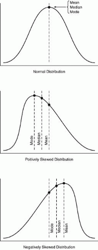 Fig. 1. Measures of central tendency. |
MEASURES OF DISPERSION
In addition to measures of central tendency, it is important to know how spread out the data set is. This is called variation or dispersion. Generally, the range, which is a measure of the difference between the largest and smallest value, provides a measure of dispersion within the data.
MEAN DEVIATION
Mean deviation is an important concept that defines the distance of the data points away from the median of the data points.
VARIANCE
Variance can be defined as the sum of the squared deviations of n measurements from the mean divided by n – 1, where n = the number of measurements, x = an individual observation, and xi = all of the subsequent data points.
Population-weighted variance:
σ2 = 1/N Σ(xi – μ)2
Sample-weighted variance:
s2 = 1/n – 1 Σ(xi – x)2
STANDARD DEVIATION
By taking the positive squared root of the variance, the standard deviation (SD) in the data set may be calculated as follows:
σ = √1/N Σ(xi – μ)2
PROPERTIES OF THE NORMAL DISTRIBUTION OR NORMAL CURVE
Using the assumption of a bell-shaped normally distributed curve, the following four important points may be noted:
Within ±1 SD from the mean value for the data, 68% of the data is contained under the bell-shaped curve,
Within ±2 SD from the mean valued for the data, 95% of the data is contained under the bell-shaped curve,
Within ±3 SD from the mean value for the data, nearly 99.5% of all the data is contained under the bell-shaped curve.
The area under the normal curve is equivalent to the probability of randomly selecting a value within that range and is equal to unity, or 1.
PARAMETRIC STATISTICS
Inferences, that is, possible conclusions, about the mean values based on a single sample can be calculated by first identifying both the null (Ho) and alternative (Ha) hypothesis. Only the null hypothesis actually is tested and refers to the fact that there is no evidence to support the hypothesis. If the null hypothesis can be rejected, then there is evidence for the alternative hypothesis (Ha). Typically, the null hypothesis is tested to a level of statistical significance in the range of p = .05, that is, the lowest range within which the null hypothesis can be rejected. Even at these levels of rejecting the null hypothesis, there is always the possibility that the null hypothesis was rejected when it actually was true. This is called a type I error. Using a possibility of p = .05 implies that the alpha (α) level is equal to .05, which means that there is a 1 in 20 chance that the data will show a significant difference when there is not one. Similarly, there is the slight chance that the null hypothesis will be incorrectly adopted when the alternative hypothesis is true. This possibility is known as a type II error or beta (β) error. In addition, it also is possible to derive the power of detecting the difference given a particular sample size. This is found using the formula (1 – β). In general, the larger the sample size, the smaller the standard error and the less the overlays between the two curves. Typically, a 10% or 20% (0.10 or 0.20) type II error is accepted.
Stay updated, free articles. Join our Telegram channel

Full access? Get Clinical Tree


