Advanced Neuroimaging Techniques for the Demonstration of Normal Orbital, Periorbital, and Intracranial Anatomy
James W. Karesh
Iftach Yassur
Marc J. Hirschbein
Advanced diagnostic imaging techniques are essential for the evaluation and management of a wide variety of pathologic processes involving facial, orbital, ocular, and intracranial structures. Improvements in both imaging hardware and software have made it possible to visualize vividly anatomical detail and physiologic processes previously possible only through a combination of surgery, gross pathologic dissection, and laboratory evaluation. The ability to reconstruct three-dimensional (3D) views of structures, to examine blood flow and inflammatory responses, and to noninvasively evaluate visually inaccessible areas from a variety of viewpoints have made these techniques integral to a physician’s medical and surgical armamentarium and vital to patient care.
During the past 30 years there have been remarkable advances in diagnostic imaging. Spatial resolution using computed tomography (CT) has improved from 4 to 0.5 mm, thus reducing the slice thickness of imaged tissue from 8 mm in the 1970s to 1.5 mm in the early 1990s.1,2 New CT scanners introduced since 1998 enable imaging that is eight times faster, with slice thickness of up to 0.5 mm.3 Through this advancement it is now possible to image such structures as the subarachnoid space around the optic nerve and individual sensory and motor nerves within the orbit. Additionally, direct multiplanar CT imaging in the coronal and sagittal planes has in many cases obviated the need for reconstructed images that invariably lack the resolution and detail of direct images.4,5,6,7 Even more recently, software advances have allowed the creation of 3D reconstructed images from thin-slice CT images.8 These include 3D reconstructions of contrast media in blood vessels, thus allowing the creation of noninvasive CT angiography (CTA). Simultaneously, during the past 10 years, magnetic resonance imaging (MRI) has achieved a level of importance at least equal to and perhaps surpassing that of CT in the imaging of orbital and intracranial structures. In part this has been the result of the decreased costs associated with this imaging modality and its more widespread availability. More important, however, is the ability of MRI to provide direct high-resolution multiplanar and 3D thin-slice images of soft tissue structures.8,9 In addition, improvements in surface coils and the introduction of fat suppression and gradient echo techniques andgadolinium-diethylenetriaminepentaacetic acid (Gd-DTPA) have further improved the imaging capabilities of MRI.10,11 As with CTA, 3D reconstructions of signals from moving protons in blood vessels have allowed the establishment of noninvasive MR angiography (MRA).
For the most part, diagnostic imaging techniques such as CT and MRI are used to obtain information about various disease states. However, to understand fully the images created by these modalities, it is essential not only to have a basic knowledge of their technical aspects but also to understand how they image normal anatomical structures. The discussion that follows is designed to help the practicing ophthalmologist understand the basic scientific and technical aspects of CT and MRI. In addition, it will include a relatively comprehensive description of the normal facial, orbital, and intracranial anatomical structures and processes imaged by these techniques.
CT
TECHNIQUE AND THEORY
The discovery of x-rays in 1895 by Roentgen ushered in the age of diagnostic imaging. The basis for the images created by x-rays is the differential absorption of such rays by various tissue structures. This is based on the fact that atoms with higher atomic numbers and greater electron density will absorb and attenuate more of these rays than those with lower atomic numbers. Therefore, for an image to be created by any x-ray imaging device, the minimal requirements include an emitter to produce x-ray energy and a detector to measure the amount of this energy transmitted through a particular structure. It was not until the 1970s, however, that a major advance was made in this area with the development of CT by EMI Ltd. of England. Since the installation of the first CT scanner in 1971, there have been four further generations of scanners that have resulted in improved spatial resolution and decreased scanning time.
In standard plain film radiography, images are produced by the exposure of a film source to x-rays transmitted through an object of study. Both the film and the radiation source are perpendicular to the object to be studied. To delineate more exactly a single plane of view, plain film tomography developed as a next step. With the use of this technique, both the radiation source and the film source are moved in synchronicity while the object to be imaged remains stationary. This enables a specific target plane to be in clear view while adjacent planes are blurred.
The development of CT represented a dramatic and significant improvement over plain film tomography. Although it also uses x-rays in an attempt to image clearly a specific object plane, its conceptual basis and methodology are markedly different. In this imaging technique a rotating radiation source is used to transmit x-rays rapidly through an object from a number of angles, usually in 1-degree increments. At the same time a rotating radiation detector array is used to measure the x-ray attenuation by a given cross section of intervening material. The data are then digitized and analyzed using various algorithms to permit gray-scale image reconstruction representing the attenuation coefficients of the imaged tissue. The algorithmic computation is simplified by using data collected from one two-dimensional (2D) slice at a time and by calculating the attenuation of many small volumes or voxels of this slice (volume averaging) instead of using data from the many points in one large volume. Image resolution is improved by reducing both the volume of a single voxel and the thickness of the individual tissue cross section through which radiation is transmitted. The unit representing the extent to which a particular voxel attenuates the x-rays is termed the Hounsfield unit (HU). The HU varies from a value of -1,000, or minimal attenuation as represented by air, to + 3,000, or maximal attenuation as represented by bone, with zero being equal to the attenuation of x-rays by a voxel of water. In gray-scale terms, the lighter the area imaged, the greater is the absorption of x-rays; the darker the area imaged, the less is the absorption of x-rays.
More recently, evolution in CT software has permitted the creation of high-resolution 3D images (Fig. 1).8 This has been of particular interest in cases of traumatic and congenital bony defects of the skull, where such images are quite useful in planning reconstructive efforts. With additional mathematical manipulation of the attenuation coefficients obtained from cross-sectional 2D slices, 3D images can be reconstructed. This is accomplished by estimating the interstice voxel HU values. These are generally assumed to be a weighted average of the HU values for the voxels of the two adjacent slices. The locations of the voxels are then described in terms of a 3D coordinate system with the z-axis parallel to the CT scanner table, the y-axis perpendicular to the top of the table, and the x-axis parallel to the CT scanner gantry opening. These images can then be reconstructed in either gray-scale or false color and recorded on film or tape.
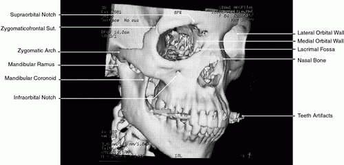 Fig. 1. Three-dimensional computed tomography reconstruction of facial bones and orbit. |
2D CT imaging is most frequently performed in the axial plane (Fig. 2). The bony anatomy of the orbit, optic canal, and intracranial cavity determines the exact orientation of this plane to provide the best visualization of both bone and soft tissue. The bony orbit is shaped like a quadrilateral pyramid lying on its side and with its base facing anteriorly. The medial orbital walls are almost parallel, although they tend to converge toward the midline in their posterior aspect. The lateral orbital walls diverge at approximately 45 degrees to the midline. The orbital axis is about 23 degrees divergent from the midline. The orbitomeatal line (Reid’s baseline or the Frankfurt-Virchow line) is an important radiologic landmark for imaging the orbital structures. It is a line that extends from the upper margin of the external auditory meatus to the inferior orbital rim. The orbital floor is at approximately a -20-degree angle with this line, and the optic canal is at approximately a -30-degree angle with this line. Axial scans of the orbit are performed parallel to the orbitomeatal line, in contrast to axial scans of the intracranial contents, which are performed in a plane parallel to the orbital roof, which is at a + 30-degree angle to this line. The optic chiasm is also best imaged in a plane parallel to the orbitomeatal line. Although both the optic canal and nerve can be adequately visualized with axial scans parallel to this plane, scans of these structures are more precisely performed if the image plane is at a -30-degree angle to this line with the globe in upward gaze. This straightens the nerve and places its axis in the same plane as the canal. The optic canal of infants and young children is at approximately a -20-degree angle with the orbitomeatal line, and in these age groups the scanning angle is appropriately modified for precise imaging of this structure. For orbital scans a 3-mm slice thickness is usually employed; for scanning the optic nerve and canal, a 1.5-mm slice thickness is recommeded to image these structures completely (Fig. 3). Thin-slice technique is helpful in reducing the effects of partial volume averaging, thus improving image resolution of small-diameter structures such as the optic nerve. In contrast, axial scans of the intracranial contents are usually 5- or 10-mm thick slices, although thinner slices are often used when imaging structures such as the cavernous sinus, suprasellar cistern, pituitary gland, and optic chiasm. Generally, the radiation dose associated with thin-cut CT imaging is 30 mGy (using 3-mm slice increments) to 80 mGy (using consecutive 1.5-mm scans), which is considerably less than complex motion tomography of the facial area and similar to standard plane film head scans.
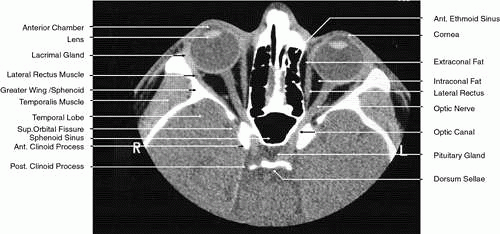 Fig. 2. Axial computed tomography scan at the level of midorbit. |
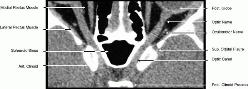 Fig. 3. Axial computed tomography scan of the orbital apex and optic canal. |
Multiplanar reconstructions are frequently used to provide imaging in the coronal, sagittal, and oblique planes in both orbital and cranial CT.12,13,14 As already noted, multiplanar reconstruction is also required for the formation of 3D images.8 These reconstructions are computer-generated from consecutive or overlapping transverse images, with the reconstructed image based on the volume (i.e., the individual voxels) of the tissue slice scanned. The resolution of these images depends on the number of slices imaged and their thickness and on the extent to which individual slices overlap. Multiplanar reconstruction is very useful in patients who cannot remain still for any length of time, who are medically or surgically unstable, who have limited mobility, or who have been injured traumatically, because this technique avoids the repositioning required for direct coronal and sagittal scanning and reduces the time needed to obtain a scan. This technique is also quite helpful when dental or other metallic appliances are present, because these items reflect or disperse radiation, resulting in significant imaging artifacts.
Direct multiplanar CT imaging provides a much improved image over those obtained through multiplanar reconstruction (Fig. 4). This technique is “slice-oriented” in that each image is obtained directly by scanning in a plane perpendicular to the tissue slice whose image is desired. In contrast, multiplanar reconstruction is “volume-oriented” in that the reconstructed images are based on the total volume of tissue imaged in one particular, usually axial, plane. Direct coronal and sagittal CT scanning requires special patient positioning that may not be possible for all patients.1,5,6,15 However, the images produced by direct scanning have significantly higher spatial resolution and quality than those produced by multiplanar reconstruction. In addition, such direct scans avoid imaging artifacts caused by eyelid and ocular movement that often occur in imaging by multiplanar reconstruction. On the other hand, imaging artifacts caused by dental appliances are often present on direct coronal and sagittal scanning. Generally, direct coronal scanning should be obtained, whenever possible, to supplement axial orbital scans to image this area most accurately (Fig. 5). Direct multiplanar imaging of the orbit and optic nerve is particularly helpful in instances of ocular and orbital trauma and in cases in which evaluation of the extraocular muscles, optic nerve, chiasm, canal, and perisellar or cavernous sinus areas is desired.
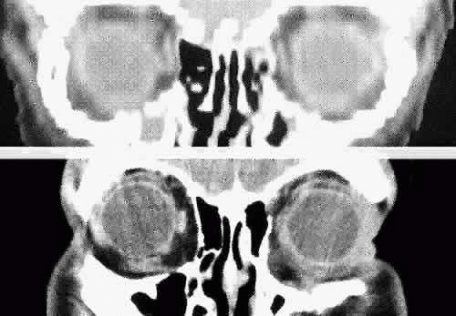 Fig. 4. Comparison of a direct coronal computed tomography scan at the level of midglobe (inferior) and coronal multiplanar reconstructions at the same level (superior). |
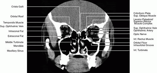 Fig. 5. Direct coronal computed tomography scan of the midorbit posterior to the globe. |
The use of intravenous iodinated contrast agents is particularly useful in showing areas of increased vascularity or breakdown in the blood-brain barrier. For these reasons it should be employed routinely when there is a need to evaluate visual loss or there is suspicion of infarction, mass lesions, inflammation and infection, or demyelinization. On the other hand, the high contrast between the vitreous, sclera, orbital fat, extraocular muscles, optic nerve, surrounding bony structures, brain, and cerebrospinal fluid reduces the need for intravenous contrast dyes in routinely imaging these structures. Generally, contrast agents are not employed in cases of intracranial, orbital, and bony trauma. In addition, further enhancement of specific structures can be obtained by manipulation of the screen image display (that is, the area scanned that appears on the technician’s video display screen is subsequently recorded onto film). To display soft tissue structures optimally, a window level between 0 and 40 HU is used, with a window width between 300 and 600 HU being most appropriate. Bony structures are optimally displayed with a window level between 40 and 300 HU and a window width between 2400 and 3200 HU.1
MULTISLICE SPIRAL/HELICAL CT AND CTA
Newer generations of scanners introduced in the last decade combined with advances in 3D imaging software and hardware have revolutionized the field of CT imaging. Multislice CT, introduced in 1998, has taken CT from an axial cross-section imaging technique to a real 3D imaging tool: near-isotropic resolution is now possible with almost identical spatial resolution along all spatial axes, including the patient’s long axis.3,16,17 As a consequence, excellent multiplanar reformats can be obtained as well as high-quality 3D reconstructions of anatomical structures.
The principal difference between multislice CT scanners and the single-slice spiral/helical scanners lies in the detector array. Two major changes were made in the scanner detectors. The detector array is configured to operate with a slip ring that allows it to rotate continuously. The rotation time for the x-ray source and detectors, formerly about 1 second for most scanners, has been reduced to 0.5 seconds. More importantly, the single detector row was replaced by four rows of detectors capable of simultaneously collecting data at different slice locations. By doubling the rotation speed and providing four times the detector rows, the data acquisition capability dramatically increases. The net is a scanner that operates four to eight times faster than its predecessors. The enhanced speed of the multislice CT scanner translates into several dramatic changes in routine practice. Because of this markedly improved speed, it is possible to choose to decrease slice thickness up to 0.5 mm to allow improved spatial resolution. Conversely, it is also possible to choose to image a larger volume and increase anatomical coverage. It is also possible to obtain images with less motion blur and artifact, decrease the need for sedation in children and noncooperative patients, decrease scanning time in trauma patients, and reduce the amount of contrast being used. Reduction in radiation exposure is also achieved. With multislice CT, there is now the option to obtain information that was not previously available. Not only axial and coronal but also sagittal images of the brain can be obtained. Thin-section scanning of the posterior fossa can be used for reduction of beam hardening artifacts and improved delineation of the brain stem.
Perhaps the most important application of spherical multislice CT is the 3D reconstructions of blood vessels that have enabled significant improvements of CTA. CTA is defined as any CT image of a blood vessel that has been opacified by a contrast medium. During spiral data acquisition, the entire area of interest can be scanned during the injection of contrast. Images can be captured when the vessels are fully opacified to show either arterial or venous phase enhancement through the acquisition of both data sets (arterial and venous). CTA acquires an entire volume of 3D data using a single injection of contrast agent. This database is then processed using special 3D software to create a 3D image of the blood vessels. Areas of interest can be retrospectively targeted and reconstructed without the need for additional iodine or x-ray exposure. Overlying structures may be eliminated by postprocessing of the image.16,17 CTA also has the ability to depict mural thrombus calcifications and true mural dimensions.
CTA of the intracranial vessels is an excellent tool for detecting cerebral aneurysm in patients with subarachnoid hemorrhage (Fig. 6). Compared with a standard cranial CT, it requires only a few more minutes to obtain detailed information about intracranial angiography. CTA obtained with multislice CT is a relatively new technology with promising implementations, but at present the clinical usefulness of multislice CT and CTA in neuroimaging is yet to be determined.
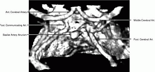 Fig. 6. Three-dimensional computed tomography angiography of the circle of Willis showing an aneurysm of the basilar artery. |
MRI
TECHNIQUE AND THEORY
The history of MR began 53 years ago when Felix Black, Edward Purcell, and other researchers laid the foundation for what has become perhaps the most complicated imaging modality of our time.18,19,20 In 1952, Block and Purcell shared the Nobel Prize in physics for their discovery. However, it was not until the development of strong superconducting magnets large enough to accommodate the human body, along with advances in computer technology, that this technology could be applied to clinical medicine in the form of MRI. In 1980, the first human MR images were produced by Hawkes and Holland and their group in Nottingham, England.21,22 Since that time improvements in MR delivery systems, the use of surface coils, the development of larger and stronger magnets as well as useful intravenous contrast agents, and reductions in the costs associated with MRI have made this technology an integral part of the physician’s diagnostic armamentarium.
MRI employs a strong magnetic field and radio waves (i.e., electromagnetic radiation in the radiofrequency range) to create tomographic sections of the human body. MRI is based on the principle that atoms having an odd number of protons spin and act as small magnets that will align in the direction of a superimposed magnetic field.8 In turn, these molecules can be influenced by an applied external radio wave to emit radiofrequency energy that can be detected by an antenna; with the use of a computer, this response can be translated into an image of a particular tissue section. This underlying theory accounts for the original name of this technology: nuclear magnetic resonance imaging. This name was changed to MRI to emphasize the fact that nuclear energy and ionizing radiation were not used as part of the imaging technique and to lower patients’ fears regarding the imaging process. The hydrogen atom is the most abundant element with an odd number of protons in living tissue and has the strongest gyromagnetic ratio. Therefore, it has the most powerful MR signal compared with other such elements. For these reasons, the MR image formed by a particular tissue is dependent on the number of hydrogen molecules present in that tissue and their response to applied radiowaves while exposed to a strong magnetic field.
To create an MR image, the patient is placed within a strong static field strength-superconducting magnet. Currently, such magnets range in strength from 1.5 to 2.0 Tesla (one Tesla = 104G; in contrast, the strength of the earth’s own magnetic field is only 2 × 10⁻⁵ Tesla). The development of these strong superconducting magnets has greatly improved the imaging capabilities of modern MR technique. The magnetic field produced by this strong static magnet aligns the patient’s hydrogen protons along the long axis of the field with slightly more protons spinning or processing in one direction (parallel along the field) than the other (antiparallel), thus resulting in a net local magnetization of the protons. The frequency at which these protons spin is directly proportional to the strength of the strong magnetic field. When a short burst of radiofrequency energy is directed at the precessing protons at the same frequency at which they are spinning, the protons will be influenced to spin in phase with each other and to emit a detectable and coherent radiofrequency signal. Although the local magnetization value of these protons is determined by the strength of the strong magnetic field, this value can be further influenced by the application of a second weak gradient magnetic field applied across the main axis of the strong magnetic field, thus changing the spin or precession of the hydrogen protons based on their location in relation to this second field. Because these protons will be spinning at different frequencies after the gradient field is applied, they will require a variety of different radiofrequency signals corresponding to these different spin frequencies to be influenced to spin in phase and to emit detectable radio waves. The location of specific protons can then be determined because both the magnitude of the weak gradient field and the frequency of the applied external radiofrequency signals are known and can be related to the emitted radio wave.18,23 In addition, the densiy of the protons responding to a particular radiofrequency signal can be determined because this is proportional to the strength of this emitted radio wave.18 The term “spin echo” was created to characterize this process in which spinning protons emit (i.e., echo) a radio wave in response to a specific radiofrequency signal corresponding to the precession frequency.24
To summarize the MR process, radiofrequency energy at a specific frequency is applied in a quick burst to a subject placed within a static strong magnetic field. Most commonly, the energy of this pulse is sufficient to rotate the local magnetic field vector of the hydrogen protons in the plane of interest by 90 degrees from the axis of the static strong magnetic field. This is termed a spin-echo pulse. For a period of time, these protons will enter a higher energy state and precess and resonate coherently at the same frequency as the applied radiofrequency energy. This coherence fades a short period after the applied radiofrequency energy is terminated, and the magnetic field vector returns to its original alignment. During this realignment, the protons move from a higher to a lower energy state, emitting energy in the form of a radio wave. This radio wave response can then be detected and the position and density of the affected protons measured. This information is then translated by computer software into a tissue image slice. Several measurements are used to characterize this process, including spin density, T1 and T2 relaxation times, and T2*, a factor related to the MR equipment.
Spin density represents the amount of free or unbound hydrogen present within a particular tissue and available for generation of an MR image. Tightly bound hydrogen does not produce an MR signal. Therefore, bone, which contains only tightly bound hydrogen, does not produce an MR signal. On the other hand, fat and water, which contain considerable unbound hydrogen, produce a significant MR signal. The amount of unbound or bound hydrogen within tissue is not manipulated during MR imaging but does determine the upper limit for signal strength. The timing and sequencing of the applied radiofrequency pulses are used to influence the greatest number of these protons to produce the strongest signal. T1, T2, and T2* are used to control the sequencing and strength of the radiofrequency signal.
After a radiofrequency pulse is applied to a subject, both the magnetization vector and the coherence of the affected hydrogen protons tend to return to their resting levels over a particular period of time. The longitudinal relaxation time, or T1, is the time it takes for 63% of the transversely rotated hydrogen protons (i.e., those protons rotated from their resting longitudinal orientation along the long axis of the static strong magnetic field) to return to this orientation. This is also the amount of time it takes before another radiofrequency pulse can be applied and a measurable signal detected. Generally, if the normal frequency of motion of a tissue’s hydrogen molecules is high, as is true with water and cerebrospinal fluid, the T1 relaxation time is long. If this frequency is reduced by the binding of water molecules in hydration layers around proteins or by dense packing of these molecules, the T1 relaxation time is shortened. On the other hand, T2, or the transverse relaxation time, represents the time it takes for 63% of these protons to lose their coherence. This is also the amount of time during which the signal from the applied radiofrequency pulse remains detectable. Generally, the more solid and compact a tissue is, the shorter the T2 time, whereas the more liquid a tissue is, the longer the T2 time. Based on the response of its hydrogen protons, each body tissue will have a characteristic T1 and T2 relaxation time in both a normal and pathologic state. Cortical bone has a low MR signal owing to its low hydrogen density, whereas rapidly flowing blood has a low MR signal because it does not remain stationary for a long enough period to produce an MR signal.
There is one additional chronologic characteristic that can be measured in MRI: the T2*.8 This is a measurement of the time it takes for a “real” MR image to disappear. The quality of the static strong magnet determines this factor, with a short T2* being inversely related to the extent of the inhomogeneities in this field. The period between radiofrequency pulses, image quality, tissue contrast, andthe persistence of the postpulse radiofrequency signals are related to this factor.
During MRI, the T1 and T2 differences between various tissues can be weighted to enhance the MR image produced. Essentially, this process increases the contrast between adjacent tissue structures and improves their visualization. This is ac-complished by varying within a particular pulse sequence either the repetition time (TR) betweenapplied radiofrequency pulses and the echo time(TE), or the time between the applied pulse andthe detection of the produced signal. A short TRfavors tissues with a short T1, such as fat. For exam-ple, with a TR of 300 msec, tissues will be enhanced in the following order: fat > white matter > gray matter > uvea > aqueous > vitreous, optic nerve, muscle > cortical bone. The reason for the intense response of fat is that with a short T1 it can almost completely recover its resting state between pulses. This enables it to respond again to the next pulse. Generally, T1-weighted images have a pulse sequence with a TR of 200 to 1,000 msec as well as a short TE (20 to 25 msec) (Fig. 7). The longer a particular tissue’s T1, the less it can respond to the next pulse, because fewer of its protons have returned to a resting state. Therefore, its MR image is less intense. Lengthening the TR will allow more protons time to relax until the signal produced no longer depends on a tissue’s T1. The image produced when the TR is long (2,000 to 2,500 msec) is “proton density”-weighted (Fig. 8). When this is the case, tissues with the highest proton density (e.g., gray matter and old hemorrhage) produce the most intense signal. In both T1- and proton density-weighted images, the TE is short (20 to 25 msec). The clearest anatomical delineation between tissues is provided by highly T1-weighted images with TR values between 300 and 500 msec.25,26
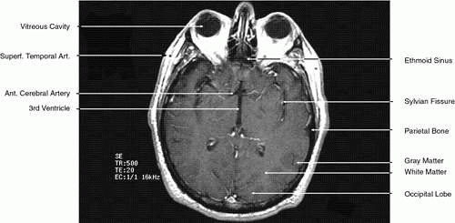 Fig. 7. Axial T1-weighted magnetic resonance imaging through midglobe. |
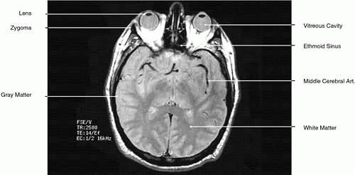 Fig. 8. Axial proton-density magnetic resonance imaging through midglobe. |
T2-weighted images can be produced at the same time as proton density images. In this case both the TR and TE are prolonged. By allowing all tissues to relax maximally, the most intense signal will be produced by the tissue with the longest T2 (that is, the tissue that remains coherent the longest). A particular tissue’s T2, which typically ranges between 25 and 150 msec, is usually much shorter than its T1. To obtain a T2-weighted image, both the TR (>2,000 msec) and the TE (50 to 150 msec) are long (Fig. 9). In such cases, vitreous and cerebrospinal fluid give the most intense images and fat, white and gray matter, bone, and air give the least intense images.
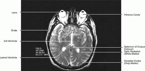 Fig. 9. Axial T1-weighted magnetic resonance imaging through midglobe. |
In addition to varying TR and TE, the sequence of radiofrequency pulses can also be manipulated to improve image contrast and clarity. Pulse sequences are usually repeated 128 or 256 or more times to achieve enough signals to form an image, with a single pulse sequence varying between approximately 0.3 and 2 seconds.26 The most common pulse sequence currently in use is the spin-echo sequence in which, as already noted, a pulse of sufficient magnitude is applied to rotate the magnetization vector of the affected protons 90 degrees from the transverse axis of the strong static magnetic field. Inversion recovery (IR) sequencing is a technique that uses a pulse of sufficient magnitude to rotate protons 180 degrees. This is followed by another pulse sufficient in magnitude to rotate these protons 90 degrees after they have partially recovered their longitudinal magnetization. Using this technique, a null signal can be obtained when this second 90-degree pulse is applied to the partially recovered protons at the time (the inversion time or TI) their magnetization vector is at the crossover point where their emitted signal can be negated. The IR technique is of particular benefit when suppression of the signal from fat is desired; in this context it has been used in orbital imaging (Fig. 10).27 However, because routine spin-echo techniques provide excellent orbital images and because the IR technique makes it difficult to separate cerebrospinal fluid from optic nerve and also creates an imaging artifact at interfaces of fat and water, this technique has not gained wide acceptance. A variety of other techniques, some still experimental, have also been developed to suppress the signal associated or in attempts to evaluate lesions associated with various degrees of vascular flow.10 However, the spin-echo technique provides a superior image to most of these and is currently the most commonly used MR technique.
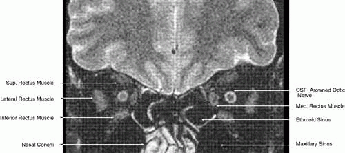 Fig. 10. Coronal fat-suppression magnetic resonance imaging through midorbit posterior to the globe. The cerebrospinal fluid cuff around the optic nerve is visible due to the suppression of the fat signal. |
Other factors are also important in ensuring that the clearest MR image is obtained.26 Most revolve around improvements in the signal-to-noise ratio (SNR). Generally, the greater the SNR, the better is the quality of the MR image. MR equipment factors, including the strength and quality of the gradient and static magnets, and the size and placement of the signal detectors (in particular, the use of small surface coils), are intimately related to image quality. Equally important is scanning technique and patient cooperation and preparation.
Except for the strength of the superconducting static magnet, the operator of the MR equipment can adjust all aspects of a particular scan, including the TE, TR, and pulse magnitude, repetition, and sequence to improve the SNR. For example, doubling the number of proton excitations will boost the emitted signal by a factor equal to the square root of 2. However, this will also double the scan time, which can lead to patient agitation and imaging artifact. The SNR can also be improved by adjusting the field of view, tissue slice, and pixel size. Normally the field of view varies between 8 and 20 cm while the size of the pixel matrix (that is, the number of pixels in the two dimensions[x, y] of the field of view) is usually 128 × 256 or256 × 256. The usual individual pixel size variesfrom 0.31 × 0.31 mm in an 8-cm field of view to1.56 × 0.75 mm in a 20-cm field of view. Thinner slices and smaller fields of view and pixel sizes are associated with lower SNRs. This is due to the reduced number of protons excited in a particular voxel and, therefore, a reduction in the signal they produce. However, if the tissues to be imaged are already small, as, for example, are the orbital structures, the spatial resolution can be improved by reducing the field of view even though there is also a subsequent reduction in the SNR. Although the SNR is linearly related to slice thickness and pixel size, it is adjusted in proportion to the square of the field of view. Therefore, all other factors being equal, a 75% reduction in SNR occurs with a 50% reduction in the field of view. On the other hand, there is a trade-off when the image slice becomes too thick. Although this will result in a linear increase in the SNR, there will also be an increase in partial volume effects with a subsequent degradation of the MR image. For MRI of the orbit, a slice thickness of 3 or 4 mm is routinely used with an interslice distance of 0.5 to 2.0 mm, whereas for intracranial imaging slice thickness of 3 to 5 mm and interslice distances of 05 to 2.5 mm are routinely employed.11 In addition, because MRI is multiplanar, direct views from several different planes (coronal, sagittal, oblique, and axial) can be obtained routinely during a single imaging session without repositioning or rescanning a patient. The SNR can also be increased by averaging the signal responses from repeated excitations of individual tissue volumes. Because this also increases the scan time and the incidence of movement artifact, especially when the eye and orbit are imaged, the number of excitations that can be performed is limited before image degradation occurs. Generally, one excitation (corresponding to 128 pulse sequences) is used for routine imaging, although signal averaging of as many as four excitations (corresponding to 1,024 pulse sequences) is possible.
The most effective method for improving the SNR for orbital imaging is with the use of surface coils for receiving emitted MR signals.28 These coils are smaller than the normal head coil and rest over the orbit. They can receive strong signals from immediately adjacent areas while limiting the signals received from more distant areas. This permits the use of thin tissue slices and smaller fields of view. Although the use of surface coils can dramatically improve the image resolution of orbital structures, the optimal depth of their use is approximately the orbital apex. The other drawback to their use is that they are more sensitive to motion artifact. For this reason, longer scans, such as T2-weighted images, can be better performed with a head coil. Several different surface coils are available. The 3-inch circular coil provides the best quality image when only a single orbit or globe is to be evaluated. A 5-inch coil can be used for evaluating structures such as the orbital apex or optic canal, but its images are only slightly superior to those that can be obtained with a head coil. A butterfly coil or binocular coil allows both orbits to be imaged simultaneously. These coils are specifically designed for orbital imaging and cannot be used for imaging other structures. They provide only a slightly less detailed orbital image than that obtained with a 3-inch coil.
Although surface coils will improve the SNR of orbital structures, sometimes the images they provide are associated with a fat signal of such intensity as to partially obscure the detail of the surrounding soft tissues. When this occurs, it may be necessary to use a fat-suppression technique such as the IR pulse sequence already described or one of several others that have also been developed for this purpose.11 In addition, it may be necessary to record the MR images onto x-ray film at two different window settings, using, for example, a wide setting (large field of view) for superficial structures with a bright signal and a narrow setting (small field of view) for deeper structures that have a less intense signal. With the use of strong superconducting magnets of 1.5 to 2.0 Tesla, surface receiving coils, and modern imaging techniques, the spatial resolution of MRI allows visualization of lesions as small as 0.4 × 0.4 × 3.0 mm3.
Unlike CT imaging, intravenous contrast agents are not routinely used in MRI. Gadolinium is a rare earth element that has paramagnetic qualities and can produce tissue enhancement by altering the surrounding magnetic environment. Although in its ionic form it is quite toxic, when chelated with DTPA it is well tolerated and can be used to enhance structures with an incomplete or absent blood-brain barrier (e.g., the cavernous sinus, pituitary gland, infundibulum, sinus mucosa, and various pathologic processes). Normal cerebral and orbital blood vessels and rapidly flowing blood will not enhance. Generally, Gd-DTPA shortens both T1 and T2 relaxation times. However, in routinely administered doses its primary effect is to shorten the T1 relaxation time. The uptake of Gd-DTPA by tissues on T1-weighted imaging results in their enhancement. However, occasionally such enhancement results in some difficulty in differentiating pathologic tissues from fat, which also enhances on T1-weighted imaging. In such cases it may also be necessary to use other imaging techniques, such as enhancing chemical shifts, to provide differentiation between normal and abnormal tissues.29
There are several relative contraindications or difficulties associated with MRI. The apparatus itself can be quite claustrophobic because patients are surrounded by the strong static field magnet during the procedure. In many cases imaging can last an hour or more, which can be quite agitating to some patients. Occasionally sedation with chloral hydrate or barbiturates may be required to allow scanning to take place and to reduce motion artifact. Another problem relates to patients with attached life-support equipment. Generally these patients cannot be scanned unless the equipment is specifically designed for use in a magnetic environment (i.e., no magnetizable materials).30 In addition, it is usually very difficult to position within an MR scanner a patient who is attached to life-support equipment. Pregnant patients may be ineligible for MRI because little is known about the effects of high-frequency energy and strong magnetic fields on the fetus. The presence of ferromagnetic metallic devices, such as vascular clips, cardiac pacemakers, and prosthetic devices, or retained foreign bodies such as those related to industrial accidents, are absolute contraindications to MRI.31,32 These devices and foreign bodies may move within a magnetic field, resulting in significant injury.33 Implants made of titanium, cobalt-nickel, or platinum (e.g., fixation plates, lens loops, retinal tacks) are not affected by MRI and are not contraindications to this process. Patients cannot wear makeup during the procedure because most eye makeup contains metallic particles that can produce significant image artifact.
Stay updated, free articles. Join our Telegram channel

Full access? Get Clinical Tree


