Adaptive Optics
Larry A. Donoso
“Imagination is more important than knowledge”
–Albert Einstein (1879-1955)
The history of ophthalmology has many parallels to the history of astronomy and astrophysics where advancements in the understanding of light or more specifically wavefront technology allowed for images of superior quality to be produced by correcting wavefront aberrations. One significant advancement in this regard is the development of adaptive optics. In astronomy, this technique has been applied to telescopes to correct wavefront aberrations, which arise from atmospheric turbulence and result in images of superior quality. In ophthalmology, wavefront correction has been primarily used in refractive surgery where the goal is to improve vision following corneal refractive surgery, possibly to the point of supernormal vision. More recently attention has been focused on the retina where it is possible to resolve single cones or cone mosaics, a technique, which may provide a means of diagnosing retinal disease at an earlier stage than conventional methodologies can resolve these pathologies as well as to monitor changes over time. This review will focus on the history of telescopes leading to the development of adaptive optics to correct wavefront aberrations and its subsequent application to ophthalmic instruments with a particular emphasis on retinal disease. It is a general review intended for clinical ophthalmologists and vision care providers who often come into contact with lenses. An excellent review of ophthalmoscopy can be found from Colenbrander,17 and an introduction to adaptive optics by Tyson.68
Telescopes – from Galileo to Hubble
Who better to introduce the topic of light and optics than with Einstein as he received, in part, the Nobel Prize for explaining the photoelectric effect (see glossary). This was an important concept in understanding the quantum nature of light and led to the concept of the wave-particle duality of light. Einstein’s quote asserts that new discoveries or innovations are based on prior knowledge. The history of not only astronomy but also of ophthalmology is brightly illuminated with innovation. One recent innovation is adaptive optics, which is being extensively used in astronomy to improve the image quality of telescopes.
Although there are a number of contenders for the inventor of the telescope (Table 1), it is Galileo who is generally given credit (although Lippershey applied for a patent one year earlier – see Timeline of Telescope Technology, www.wikipedia.com.). He created a telescope capable of observing never before seen mountains and valleys on the moon. His telescope consisted of a straight tube with lenses, thus it was a refractive telescope and has been called a Galilean telescope. Later Newton improved on this design by introducing a mirror to improve image quality, thus creating a reflective telescope (Newtonian telescope).
Table 1 – History of the Telescope | ||||||||||||||||||||||||||||
|---|---|---|---|---|---|---|---|---|---|---|---|---|---|---|---|---|---|---|---|---|---|---|---|---|---|---|---|---|
| ||||||||||||||||||||||||||||
Image quality was of concern to Sir Issac Newton as well, in part, due to the observation of the twinkling of stars. Newton in the early 1700s realized that stars twinkle because of impurities in the earth’s atmosphere. It was an amazing observation since, in general the universe (not the earth’s atmosphere) acts like a vacuum where light travels at a constant velocity of approximately 186,280 m/sec 50. This approximation is true until light enters the earth’s atmosphere where is it slowed down by atmospheric turbulence to approximately 185,250 m/sec, or one million billionth of a second from traveling from the sun to the earth’s surface.
It is this property, atmospheric turbulence (Fig. 1) that is of great concern to astronomers even today. Atmospheric turbulence refers to, among other things, the different temperature layers and wind speeds of air in the atmosphere. These differences in properties of air distort the light wavefronts leading to aberrations in the image of a star including what we commonly call twinkling (the less or more dense layers refract light towards or away from the observer – hence the star appears to twinkle). In astronomy, the absence of atmospheric turbulence may give rise to what is commonly referred to as “good seeing,” a general description that refers to image quality (like visual acuity or air pollution index) and can be measured in terms of the ability to resolve an image (units are usually in arcseconds or how many degrees apart an image can be resolved). Seeing is a critical concept in astronomy since both optics and the earth’s atmosphere determine the resolution of a telescope, particularly large telescopes.
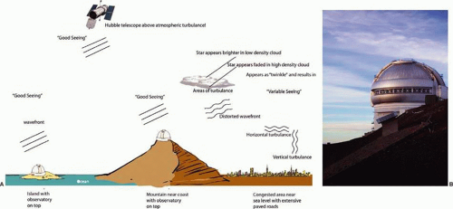 Figure 1. A. Atmospheric turbulence. Turbulance in the atmosphere occurs under different conditions. In the atmosphere approximately 5 miles above the earth’s surface the air is subject to temperature gradients and high wind velocities and generally causes what is referred to a horizontal turbulence. Near the earth’s surface there is a drag caused by air friction against the ground. In addition, heat that is generated by, for example, paved roads around telescopes may cause vertical turbulence. For these reasons, and others, telescopes are often located on mountain tops and adjacent to oceans with cooling winds and are painted white (see Fig. 12A) or silver (B). One way to avoid turbulence is to place a telescope, such as the Hubble Space Telescope (HST), above the earth’s atmosphere (about 370 miles up). It is turbulence that allows for what astronomers call “seeing” and in areas of high- or low-density stars can refract light towards or away from us resulting in “twinkling.” Seeing can be quantified in arcseconds (subsection of a circle) as the diameter of a star image caused by atmospheric turbulence. Hence, good “seeing” is observed in conditions of little or no twinkling, perhaps somewhat analogous to good or bad visibility in fog or perhaps vitreous opacity. The significance of atmospheric turbulence is that both optics and the earth’s atmosphere determine the resolution of a telescope, particularly a large telescope. As shown in the diagram, in areas of good or ideal seeing the incoming wavefronts are parallel, whereas in areas of variable seeing the incoming wavefronts are distorted. The goal of adaptive optics is to correct the distorted wavefront (in a closed loop system) in order to achieve “seeing” conditions and images that can be obtained above the earth’s atmosphere like the HST. B. Silver dome of the Gemini observatory operated by a consortium of seven countries and located atop Mauna Kea, Hawaii. The complex consists of 13 telescopes funded by 11 countries. Photograph provided by Richard Wainscoat. Mauna Kea is unique as an astronomical observing site. The atmosphere above the mountain is extremely dry, which is important in measuring infrared and submillimeter radiation from celestial sources, and cloud-free, so that the proportion of clear nights is among the highest in the world. The exceptional stability of the atmosphere above Mauna Kea permits more detailed studies than are possible elsewhere, while its distance from city lights and a strong island-wide lighting ordinance ensure an extremely dark sky, allowing observation of the faintest galaxies that lie at the very edge of the observable Universe. A tropical inversion cloud layer about 600 meters (2,000 ft) thick, well below the summit, isolates the upper atmosphere from the lower moist maritime air and ensures that the summit skies are pure, dry, and free from atmospheric pollutants. From www.ifa.hawaii.edu. |
The brilliant Russian mathematician Kolmogorov,66 best known for his probability theory, developed a model of turbulence, which is still in use today6,7,37,41,67,73 One effect of atmospheric turbulence is that it generally decreases exponentially with altitude and that is one reason for locating astronomical observatories on mountain peaks (Fig. 1), well above the Earths surface layer. Jets try to fly in the stratosphere (around 10 miles above the earth’s surface) because of less turbulence. Laser guide stars, which serve as artificial distant “stars” for optical telescopes14,15,19,21,22,24,27,28,30,34,39,40,43,52,57,60,70,71 are located about 50 miles above the earth’s surface.
In recent history, perhaps no greater achievement in optics was made than that of the Hubble Space Telescope (HST) (Table 1), which was placed into the outer reaches of the Earth’s atmosphere in 1990 (Table 2). The telescope orbits approximately 350+ miles above the earth at a height where superior images can be obtained because of the lack of atmospheric turbulence, hence optimal “seeing.” The telescope is composed of two aspheric mirrors. The primary mirror is approximately 7 feet (2.4 m) in diameter. The Pointing Control System (PCS) aligns Hubble so that the telescope points to and remains locked on a target. The PCS is designed for pointing to within .01 arcsec and is capable of holding a target for up to 24 hours while Hubble continues to orbit the Earth at 17,500 mph. If the telescope were in Los Angeles, it could hold a beam of light on a dime in San Francisco without the beam straying from the coin’s diameter (hubble.nasa.gov). The Hubble telescope was named after Edwin P. Hubble, a noted astronomer who conducted extensive research into stars and galaxies and was the first to show that the universe is expanding based on the concept of a red shift (see glossary).33,38 Notable achievements of the Hubble telescope include investigations of planets, super stars, and dying stars (Fig. 2). Other achievements include; in June 1994 NASA releases Orion Nebula images that confirm the births of planets around newborn stars; in November 1995 NASA released Eagle Nebula images showing where stars are born; in January 1996: NASA releases the “Deep Field” images in which Hubble peers back in time more than 10 billion years and revealed at least 1,500 galaxies at various stages of development; and in February 2001 images of the “ant nebula.” Because the Hubble telescope provides optimal “seeing” but is expensive to construct (over $2 billion) and maintain, other systems, including adaptive optics, have been developed to, in effect, create a “Hubble on Earth.”
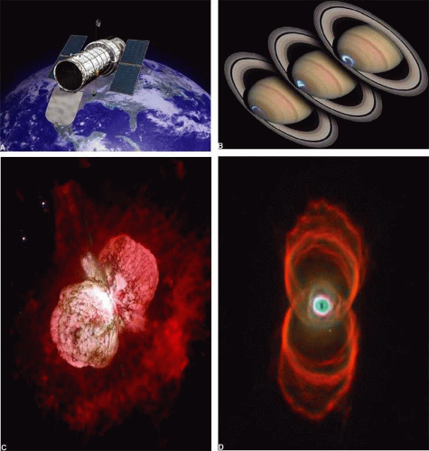 Figure 2. Hubble Space Telescope. A. Hubble Space Telescope in orbit. B. Saturn (the ringed planet). C. Etacarina (a superstar several million times brighter than the Sun; 8,000 light years away). D. Hourglass (dying star, a planetary nebula). (Images provided by NASA, except (A) that is an istock photo). |
Table 2 – Layers of the Atmosphere | |||||||||||||||||||||
|---|---|---|---|---|---|---|---|---|---|---|---|---|---|---|---|---|---|---|---|---|---|
| |||||||||||||||||||||
In this regard, Horace W. Babcock in 1953 published the first manuscript describing the concept of compensating astronomical seeing, the forerunner of adaptive optics. Babcock reasoned that it would be possible to compensate for the atmospheric turbulence causing the distortions in quality of astronomical images or “seeing” as mentioned above. An adaptation of his historic concept is shown in Figure 3. In essence, a closed loop or feed back system continually monitors wavefront aberrations and applies a “compensation” to correct for the distortion whereby the resulting image approaches a near “perfect” image or at least an image free of distortions caused by atmospheric turbulence. Not only was improved seeing beneficial to astronomy but it also had implications in the so-called Star Wars Initiative at this point in time as well. Today adaptive optics has implications for almost anything that involves a waveform (Table 3) from Atmospheric turbulence to Z-wave technology.
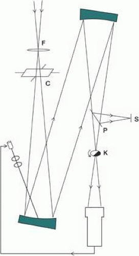 Figure 3. Babcock’s “Seeing Compensator.” The diagram adapted from the original manuscript where F corresponds to the objective lens of the telescope receiving the incoming light from the star; C is the equivalent of a tilt-tip mirror. The heart of the system are two parabolid off axis mirrors of which one is covered by oil and can be electrically charged and thus manipulated The electric charge corresponds to the image that can centered on a knife edge (K), transmitted to a cathode ray tube to be analyzed and corrected by the analyzer and returned to the system, thus completing the feed back loop. In essence, this system allows for sampling of the incoming wavefront, analyzing for wavefront distortion represented by an electric charge, compensating for the electric charge and then resampling the correction after refocusing on the knife edge and observing the corrected image at P and S. |
Table 3 – Examples of Wave Forms | ||
|---|---|---|
|
Ophthalmoscopes – from Helmholtz to Hubble
Advancements made in astronomy, including adaptive optics, did not go unnoticed by the ophthalmic community. After all, the human eye is an ultra refined optical system as well. A major difference between modern telescopes and the human eye is that the large telescopes gather in more light for image viewing because of their mechanical makeup. In perspective, a telescope can resolve objects about 1/60 the size that the human eye can. For example, an average telescope can resolve a pair of car headlights about 60 miles away (www.cfht.hawaii). Perhaps one major difference between ophthalmology and astronomy is the use of optics to completely change how surgical procedures are done. Of particular note is the use of microsurgical instrumentation.63 These advancements were largely due to Carl Zeiss and Ernst Abbe whose innovative techniques in the manufacture of optical quality glass revolutionized the making high quality optical instruments useful for many scientific disciplines including both astronomy and ophthalmology (see www.company7.com). The optical paths for various ophthalmic instruments frequently used in ophthalmology are shown in Figure 4. However, an excellent review is provided by Colenbrander.17 In brief:
Ophthalmoscope, Direct
Although originally invented by Charles Babbage in 1847, it was not until it was independently reinvented by Hermann von Helmholtz in 185136 that its usefulness was recognized.
While training in France, Andreas Anagnostakis, MD, an ophthalmologist from Greece, came up with the idea of making the instrument hand-held by adding a concave mirror. Liebreich created a model for Anagnostakis, which he used in his practice and subsequently was presented at the first Ophthalmological Conference in Brussels in 1857 and soon became very popular among ophthalmologists.
In 1915, William Noah Allyn and Frederick Welch invented the world’s first hand held direct illuminating ophthalmoscope (cited at www.hoovers.com) (Fig. 4), precursor to the device now used by clinicians around the world. This refinement and updating of von Helmoltz’s invention enabled ophthalmoscopy to become a standard medical screening device. The company started as a result of this invention is Welch Allyn. Arguably, this is the most utilized optical instrument in ophthalmology in the world today.
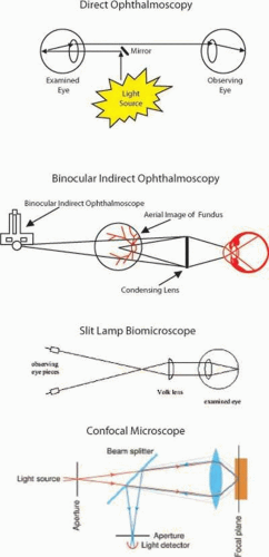 Figure 4. Diagram of light path of common optical instruments. A. Direct ophthalmoscope. B. Binocular indirect ophthalmoscope. C. Slit lamp biomicroscope. D. Confocal microscope. |
Ophthalmoscope, Indirect
In 1945, Charles Schepens invented the indirect ophthalmoscope which, in contrast, to the direct ophthalmoscope produces a stereoscopic view of the fundus of the eye. This allowed Dr. Schepens to examine his retinal detachment patients following surgery in a manner that could not have been done before and has now become one of the traditional instruments used in ophthalmology (Fig. 4). His original instrument is part of the Smithsonian Collection (Retina Society; 2003). A similar technique for observing the retina and the posterior of the eye can be accomplished with a hand held lens at the slit lamp (Fig. 4).
Retina Fundus Camera
In 1925, Zeiss marketed the first retinal camera, which was practical to use (www.company7.com). This innovation in optics preserved images of the eye, which were otherwise only captured by an artist.
Fluorescein Angiography
In the late 1950s Novotny and Alvis published their results of imaging the retina with the new technique of intravenous fluorescein angiography (IVFA).54 Novotny and Alvis were in medical training at the University of Indiana and were studying the oxygen saturation in retinal arterioles. The first analysis was on a drop of blood from Dr Alvis, and the first IVFA came after being injected with fluorescein (Fig. 5). They reasoned that fluorescein would make it easier to determine levels of oxygen saturation in the blood.
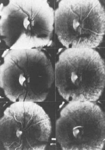 Figure 5. The first fluorescein angiogram. Fundus photograph of the eye of Dr. Alvis in the late 1950s. (From www.opsweb.org, courtesy of the Indiana University School of Medicine, Department of Ophthalmology). |
Both the Scanning Laser Ophthalmoscope and Optical Coherence Tomography scanners have recently made use of adaptive optics that can provide resolution to a single cell or in three dimensions.
Scanning Laser Ophthalmoscope
The scanning laser ophthalmoscope came into being in the 1980s followed by three dimensional images of the retina using optical coherence tomography. Color imaging using a scanning laser ophthalmoscope was introduced by the John Forrester research group in Aberdeen, Scotland, in 1998.47 This technique took advantage of the conventional monochromatic imaging system of the eye coupled with blue, green and red laser. This instrument allows for the imagining of thick specimens, lower light intensities and can allow for three-dimensional reconstruction of complex tissue such as the retina (Fig. 6).
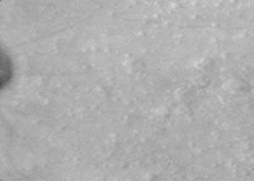 Figure 6. Scanning Laser Ophthalmoscope (SLO). Macular drusen: Drusen are waste products of metabolism accumulated under the retina. Drusen are associated with age-related macular degeneration and they appear as yellow spots. If they are buried under a layer of tissue, then they are not easily detected. With SLO, it is possible to clearly see them in the indirect mode where a confocal aperture allows only scattered light. (From www.abdn.ac.uk). |
Optical Coherence Tomography
Optical Coherence Tomography or OCT has gained wide spread popularity in ophthalmic imaging in the last few years, particularly for examination of retinal tissue (Fig. 7). For reviews, see.1,10,12,35,51,65,77,82 It was first devised in 1991 by Huang et al.,32 and is a non-invasive imaging technique based on interferometry. Hence, it is reasonably inexpensive and does not carry risks associated with invasive diagnostic procedures. As such, it is well suited for not only ophthalmic uses but also dentistry, dermatology, endoscopy, gastroenterology, and intra-arterial imaging In essence, the technique is based on light interference and can be thought of as a series of A and B scans combined to obtain a cross-sectional image with volume. The images obtained by this technique are of higher resolution than by ultrasound, but OCT penetrates to less tissue depth. The main types of OCT that exist at present include Time Domain OCT, Frequency Domain OCT (FD) or Fourier Domain. Fourier Domain OCT offers the advantage of speed, resolution and sensitivity. It is, however, a rapidly changing field as Fourier Domain 3D OCT scans have now emerged. The limits of this technology are yet to be determined particularly with regard to resolution.
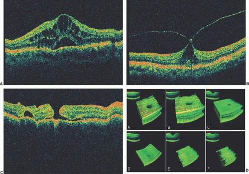 Figure 7. Composite of OCT use in retinal disease. A. Cystoid macular edema. B. macular pucker. C. macular hole. D. 3D image of various sections through the retina). (A, B, and C are courtesy of Jay L Federman, MD, with permission; D is courtesy of the University of Cardiff, UK, School of Optometry, Biomedical Imaging with permission). |
Components of an Adaptive Optical System
There are similarities and differences between astronomical “seeing” and visual “seeing” and are depicted in Figure 8. In this regard, both systems represent a closed loop system and contain a lens or lenses. The atmosphere in space is analogous to the vitreous of the eye. The retinal rods and cones and wavefront sensors are stimulated by incoming wavefronts either in parallel or aberrated. The optic nerve acts like electrical wires and the brain and computer analyze data including making decision about how to react to the data. The basic components of the adaptic optics system consist of: a wavefront sensor, a deformable mirror, and a high speed computer and other ancillary equipment and the components vary slightly when speaking of a telescope or an eye (Fig. 9).
Stay updated, free articles. Join our Telegram channel

Full access? Get Clinical Tree


