Quantifying Fundus Autofluorescence
Dietrich Schweitzer
INTRODUCTION
The investigation of endogenous fluorophores has the potential to aid in evaluating the metabolic status of tissues and thus detecting the early stages of disease (1,2). The redox pairs of fluorophores, the coenzymes NAD-NADH (oxidized and reduced forms of nicotinamide adenine dinucleotide) and FAD-FADH2 (oxidized and reduced forms of flavin adenine dinucleotide) are electron transporters in the basic processes of cell metabolism (Fig. 8.1). NAD and FAD participate in reactions that occur in β-oxidation of fatty acids (acyl-CoA-dehydrogenase reaction), in glycolysis, in the citrate acid cycle (succinate dehydrogenase reaction), in the respiratory chain in complex I (NADH+ + H+ ubichinone reductase) reactions, in the succinate dehydrogenase reaction in complex II reactions, and in the connection between the citrate acid cycle and the respiratory chain (3).
It appears that the dominant fluorophore of the fundus is the aging macular pigment lipofuscin, which appears to play an important role in the pathophysiology of several retinal diseases, including age-related macular degeneration (AMD) (see also Chapters 2 and 3). Other fluorophores include advanced glycation end-products (AGEs), which are involved in the pathogenesis of diabetes mellitus; elastin and collagen, which change during sclerotic processes and in glaucoma; pyridoxal phosphate, the prosthetic group of all amino transferases; protoporphyrin IX, a fluorophore in hem synthesis; and the amino acids tryptophan, kynurenin, and phenylalanine, which are strong fluorophores in connective tissues and the cornea, lens, and sclera (4) (see also Chapter 3).
Since an evaluation of the metabolic status of tissues requires information on single fluorophores, however, the separation of individual signals corresponding to each of these fluorophores from within the sum of the fundus autofluorescence (AF) signal represents a challenge. This chapter reviews possible methods to achieve that goal, as well as their limitations.
METHODS FOR DISCRIMINATION OF FLUOROPHORES
According to the chemical structure, there are three characteristic properties—the excitation spectrum, the emission spectrum, and the fluorescence lifetime after excitation by short pulses—that allow discrimination of fluorophores (5). In the eye, the spectral range for examination is limited to between 400 and 900 nm by the transmission of the ocular media in the short-wave range and the absorption of water in the long-wave range, respectively (6). The decrease in the ocular transmission, which occurs with increasing age, can be determined (7).
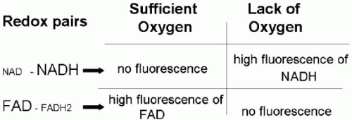 FIGURE 8.1. Change of fluorescence of coenzymes NAD and FAD depending on the availability of oxygen. |
Since specific excitation maxima are shorter than 400 nm, a differentiation of the fundus fluorophores is limited according to the excitation spectra. If the sample can be strongly excited and the fluorescence signal can be detected with a high signal-to-noise ratio, the contribution of single fluorophores can be recalculated in the sum emission spectrum. In such a fitting procedure, the spectral course of the emission spectra of each fluorophore must be known. Weighting factors are optimized until the approximation of the model function and the measured sum fluorescence spectrum are optimal. These weighting factors correspond to the contribution of each fluorophore to the sum spectrum. The signal-to-noise ratio is equal to the square root of the collected number of photons. To obtain a high number of photons, the irradiance must be high or the measuring time will be long. Generally, spectral intensity measurements suffer from absorption and scattering in nonfluorescent substances, which weaken the excitation light and change the spectral shape of the emission spectrum.
The fluorescence lifetime, the third parameter for discrimination of fluorophores, has some important advantages. The lifetime is independent of the absorption or scattering of neighboring substances. There is also no dependence on the concentration of fluorophores. Weakly emitting fluorophores can be separated from strongly emitting fluorophores if the lifetimes are sufficiently different. Only about one hundred photons are necessary for approximation of a monoexponential decay (8). Because the lifetime depends on pH value and viscosity, information can be found related to the cellular embedding matrix.
Limiting Conditions for Measuring Fundus Fluorophores
There are some limiting conditions that must be taken into account in two-dimensional (2D) measurements of fundus fluorophores in vivo:
The fundus fluorescence is covered by the strong fluorescence of the anterior segment of the eye. The techniques of aperture division and confocal laser scanning can reduce the influence of fluorescence of, cornea and lens (see also Chapters 3 and 5); a combination of both methods is advisable for accurate measurements (9). The emission spectra of the lens and cornea are minimal for wavelengths longer than 570 nm (10), and thus their influence will be reduced when long waves are used.
Endogenous fluorophores are present in all layers of the fundus.
The strong fluorescence of lipofuscin covers the weak fluorescence of other fluorophores.
Eye movement limits the time available for highly spatially resolved measurements.
The maximal permissible exposure (MPE) is the most important limitation for spectral measurements in the eye (11).
Fluorescence Lifetime Measurements
Lifetime measurements are best suited for detection and discrimination of fluorophores in images of the fundus. There are two methods for detecting fluorescence decay: measurement in the frequency domain or measurement in the time domain (5).
Fluorescence Lifetime Measurements in the Frequency Domain
In the frequency domain, the sample is excited by intensity-modulated light. The emitted fluorescence light is also modulated. There is a phase shift between excitation and emission light because of the delay between absorption and emission. This phase shift depends on the modulation frequency. The modulation in the fluorescence light is also weaker than the excitation light and decreases with increasing modulation frequency.
From the phase shift, the fluorescence lifetime τp is determined according to the following equation:
where Φ = phase shift and ω = modulation frequency.
The lifetime τm, as determined from demodulation measurements, is calculated by:
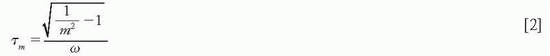
where m = demodulation.
The demodulation m is determined by the ratio of maximal and minimal intensity in the emitted light, divided by the ratio of the maximal and minimal intensity in the excitation light. The same values (τp = τm) are determined in monoexponential decay, but in multiexponential decay they are τp < τm. In the case of multiexponential decay, the decay times are calculated according to the complicated set of formulas (12):
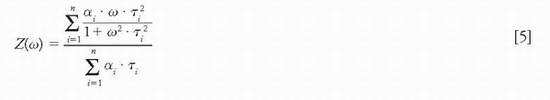
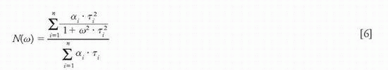
The lifetimes τi and the pre-exponential factors αi of the component i are calculated iteratively, not analytically.
In principle, one can determine the fluorescence lifetimes simultaneously for all image pixels by illuminating the whole image and detecting phase shift or demodulation using a detector matrix. Sequential excitation of all image pixels can be achieved with the use of a scanning system with only one detector. A combination of both methods is also possible.
Fluorescence Lifetime Measurements in the Time Domain
Fluorescence lifetime measurements are performed in the time domain by exciting the sample by pulses having a short full width at half maximum (FWHM), e.g., in the pico- or femtosecond range. Because the decay of the fluorescence is too short for direct measures to be obtained, the fluorescence intensity is detected during multiple excitations in a number of time windows, in a single variable time window (boxcar principle), or by time-correlated single photon counting (TCSPC). In TCSPC, the sample is excited by weak light pulses. The intensity is so low that only one photon will be detected in a sequence of about 10 excitation pulses. Each fluorescence photon will be accumulated in time channels according to the detection time after the excitation pulses. After a sufficient measuring time, the content of all time channels represents the probability density function of the decay process. The principle of TCSPC, technical details, and practical applications were previously explained by Becker (13).
The process is mostly assumed as an exponential decay, which can be approximated by a sum of e-functions:
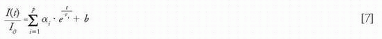
where αi = preexponential factor of exponent i or amplitude, τi = lifetime of exponent i, b = background, and p = degree of exponential function.
Because the excitation is not a Dirac pulse, the measured decay of fluorescence is the convolution of excitation pulse with the decay process. Therefore, the criterion for the fitting process is the minimization of Χr2:
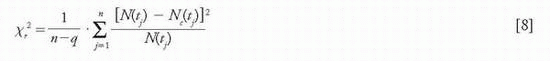
In this equation, N(tj) is the measured number of photons in the time channel j; NNc(tj) is the number of expected photons, which are calculated by the convolution of the instrumental response function and the model function; n is the number of time channels; and q is the number of free parameters (αi, τi, b).
If the detection of photons is a Poisson process, the mean square root error between detected photons and calculated photons is equal to the square root of the detected events:
Thus, the ratio in the sum of Eq. [8] is one for each time channel and the sum is n. This means that the limiting value of Χr2 is one. The algorithm is independent of the degree of exponential function, but the calculation time increases with the number of exponents. The time between two excitation pulses should be about five times the longest expected decay time.
The separation of fluorophores can be improved by global analysis (14). In this analysis, at least two data sets are considered that contain the same fluorophores, characterized by the decay time, but have different contributions αi.
In addition to discrete e-functions, other models can describe the distribution of lifetime in complex systems, including the lifetime distribution (15), stretched e-function (16), time-resolved area-normalized emission spectroscopy (17), and Laguerre expansion techniques (18).
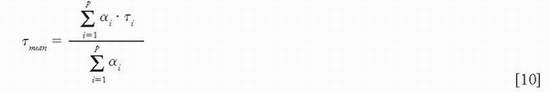
For evaluation of lifetime measurements, in addition to the single amplitudes and lifetimes, the parameters mean lifetime τmean and relative contribution Qi are helpful. Here the mean lifetime is defined as:
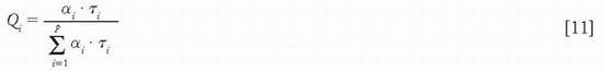
The relative contribution Qi of the component i corresponds to the area under the decay curve, determined by the component i. This value is calculated according to:
Two-dimensional lifetime measurements can be performed in scanning systems, with a pulse laser used as the light source. In contrast to applications in microscopy, the movement of the object eye must be detected and compensated for. The correct relation between detected photons and the position in the sample can be determined by the control signals, the frame and line clocks, and the (line) timer signal. The time between the excitation pulse (sync signal) and the detection time of the first and unique photon is used for allocation in the time channel. If there are multiple detectors in different spectral channels, differences in the fluorescence spectra can be used for further differentiation of fluorophores, e.g., by global fitting. In addition, fluorescence spectra can be reconstructed from the photons detected in each spectral channel.
Starting from the MPE of the eye, lifetime measurements in the time domain were optimally suited for measuring the dynamic AF of the fundus (19). Only a weak excitation power is required for detection of signal in TCSPC. This technique offers the most sensitive detection of light. To ensure a high number of photons, which is required for a good signal-to-noise ratio, the photons are added from a series of single image measurements after image registration.
STUDIES ON ISOLATED FLUOROPHORES
Excitation and Emission Spectra of Expected Fundus Fluorophores
Stay updated, free articles. Join our Telegram channel

Full access? Get Clinical Tree


