Group
Definition
Training data set
Test data set
Visual field
Evaluation of optic disc photographs
“Erlangen Glaucoma Registry”
Outpatient department of “Erlangen University Eye Hospital”
Losses (octopus)
Number
Age [years]
Number
Age [years]
Control
No
Normal
161
53.8 ± 10.2
93
55.6 ± 6.0
Preperimetric
No
Glaucomatous
102
55.8 ± 9.7
47
56.5 ± 6.3
Glaucoma
Optic disc
Perimetric
Yes
Glaucomatous
130
55.6 ± 8.9
55
58.3 ± 5.2
Glaucoma
Optic disc
3.2.2 Subjects and Patient
Controls: The reference sample included randomly selected eyes of healthy control subjects from the Erlangen glaucoma registry. The control subjects of the test sample were healthy chaperons of patients or patients of the University Eye Hospital who had treatment (e.g., cataract surgery, no glaucoma) in the second eye. In all control eyes of this study, slit-lamp inspection, perimetry, tonometry, funduscopy, and papillometry were normal.
“Preperimetric” glaucoma patients: In the “preperimetric” glaucoma groups, patients showed glaucomatous abnormalities of the optic disc. Computerized visual field examinations with white-on-white perimetry were normal. The results of measurements on one randomly selected eye of each patient were used in the study.
“Perimetric” glaucoma patients: All patients of these groups had glaucomatous optic disc damage and pathological cumulative perimetric defect curves, i.e., local and/or diffuse visual field loss in white-on-white perimetry. Visual field losses of conventional white-on-white perimetry (Octopus standard index; perimetric mean defect) were 6.9 ± 5.3 dB in the training and 7.1 ± 4.2 dB in the test population. In both perimetric glaucoma groups, one eye of each patient was selected for the assessment of validity; this was always the eye with more advanced perimetric loss.
3.2.3 Screening with FDT Perimetry
The FDT perimeter (Zeiss Humphrey Systems) tests local contrast sensitivity in the central visual field. The technique has been described as a helpful test for diagnosing glaucoma [14, 21–23]. The device uses the frequency doubling phenomenon: if a low-spatial-frequency sine-wave grating pattern (0.25c/deg) is alternated with a temporal high-frequency (25 Hz) counter-phase flicker, the spatial frequency seems to be double that of the actual spatial frequency. In the present FDT test strategies (C-20-5 or N-30-5), this stimulus is presented in one of 17 target locations on a random basis. In the software version N-30-5 of the FDT perimeter, two more test locations are studied in a separate step of the test procedure. These additional tests are not considered in the present evaluation. The stimulus presentation consists of four targets per quadrant approximately 10° in diameter and one central 5° radius target. Each stimulus was presented maximally 0.4 s on a screen with a constant time-averaged luminance (100 cd/m2). The interstimulus interval was variable in order to reduce anticipation and rhythmic responses by the patient. Two types of catch trials were generated to attract the subject’s attention and to obtain an impression of the goodness of the fixation. A 1-degree catch trial pattern at the location of the optic disc and a zero-contrast false-positive catch trial were randomly presented three times each. Subjects with more than one of the six catch trials positive were not included in this study, but the test was repeated. Before testing with the FDT perimeter, the subjects were shown a card with examples of the gratings to make them familiar with the test location and the stripe pattern. During the test, all other light sources, except the control monitors, were switched off in the examination room and a learning procedure was run. Patients were instructed to fixate the square target in the middle of the FDT screen and to press a response button if the flickering stripe pattern appeared anywhere on the monitor. Both eyes of the subjects were examined using the screening program C-20-5 with a 2 min rest period between the first (right) and second (left) eye [24]. This procedure presents stimuli with a contrast that 95 % of the normal population of the corresponding age group is able to detect. If the stimulus was detected, it was assumed that contrast sensitivity is within normal limits, and no further testing was performed at that location. If the initial stimulus was missed, the same stimulus was presented at that location a second time. If it was missed again, the instrument presented a stimulus with a contrast detectable by 98 % of the normal population, and if this was missed, a stimulus with a contrast detectable by 99 % of the normative subjects was presented. This strategy allows generating a score ranging from zero (i.e., first presentation seen) to four (i.e., 99 % level not seen) for all test locations. Considering all fields, the score ranges from 0 to 68 and from 0 to 16 in single quadrants [25]. The total FDT score is given for all groups in Table 3.2.
Table 3.2
Results of the subjects in all subgroups of the study: the overall defect score in FDT perimetry and measures of the optic disc (total size of the optic disc and the area of the neuroretinal rim)
Group | Training data set | Test data set | ||||||
|---|---|---|---|---|---|---|---|---|
n | Disc size [mm2] | Rim area [mm2] | FDT score | n | Disc size [mm2] | Rim area [mm2] | FDT score | |
Control | 161 | 2.25 ± 0.51 | 1.59 ± 0.29 | 0.6 ± 1.40 | 93 | 2.29 ± 0.53 | 1.57 ± 0.3 | 0.45 ± 1.1 |
Preperimetric | 102 | 2.45 ± 0.53 | 1.34 ± 0.31 | 4.2 ± 7.1 | 47 | 2.46 ± 0.46 | 1.39 ± 0.27 | 1.7 ± 2.9 |
Glaucoma | ||||||||
Perimetric | 130 | 2.37 ± 0.48 | 1.02 ± 0.32 | 28.3 ± 18.3 | 55 | 2.36 ± 0.55 | 1.04 ± 0.36 | 28.7 ± 20.1 |
Glaucoma | ||||||||
3.2.4 Heidelberg Retina Tomograph (HRT)
The Heidelberg Retina Tomograph (HRT I or HRT III for the reference sample, HRT II for the test sample), which generates stereometric measurements of the optic nerve head, was used to examine the morphology of the optic nerve head. A series of confocal images is obtained at consecutive focal planes and converted by the HRT software into a single tomographic image. To allow inclusion of results from the earlier HRT machines, we reanalyzed all data using the HRT III software which is backward compatible to earlier versions. To analyze the morphology of the optic nerve head, we included parameters derived from HRT images both globally and within six sectors as pre-given by the HRT. Several more newly given parameter of the HRT (e.g., steepness of the rim, glaucoma probability index) had been omitted in the present calculation because these parameter were not available in all data sets. The sector-related and global standard HRT parameters characterize volume and area of the neuroretinal rim, steepness of the cup (third moment), mean and peak height of the contour line, its height variation, the maximum depth of the cup, the papilla radius, and further volume and surface measures. The analysis includes linear discriminant formulas [26] (FSM-LDF, RB-LDF) and a score considering MRA classification in six sectors ranging from 0 to 12. Results in normal subjects and different glaucoma groups have been published earlier [27, 28]. In addition we tested a “corrected rim area” taking into account the dependency of the rim areas on the size of the optic disc [11, 29, 30] and the age of the subject similar to what was suggested earlier (Moorfields regression analysis). Instead of the originally published equation [11] which is recommended for subjects with optic discs between 1.2 and 2.8 mm2, we used a slightly modified formula as in our subjects the range of the optic disc size was larger. For calculation of the present correction formula of the rim areas, we used all the data of 480 healthy control eyes available from the Erlangen glaucoma registry. In this control group, the equation used for the correction of the rim size was: rim area = 1.2424 + 0.206 (disc area) − 0.003 (age). Figure 3.1 shows the relationship between neuroretinal rim and disc area for all control subjects of the Erlangen glaucoma registry using the present correction of the rim area. For the calculations in the present analysis, the patients with optic disc areas smaller than 1.3 mm2 and larger than 3.7 mm2 were not included because such values were not in all groups.
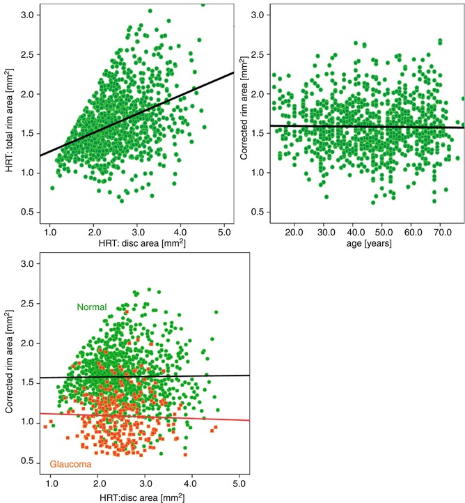
Fig. 3.1
Rim area versus disc area for all control eyes of the Erlangen glaucoma registry (upper, left). Upper right and lower plot: Middle, right: the same population after correction for disc size and age using the regression equation (“corrected rim area” = a * rim area/(b * disc area − c * age)). A group of glaucoma patients (red symbols) is included in the right lower figure to visualize the usefulness of this method in patients. A subgroup (see present inclusion criteria) of this normals and patients serves as learning cohort. HRT Heidelberg Retina Tomograph
3.2.5 Automated Classification
In total, 112 variables were used to train the random forest classifier. We used four FDT sector scores, one overall FDT score, four sector differences and the upper/lower hemifield difference as FDT variables, and 102 HRT variables obtained from the instrument for the combined classifier. A second classifier using the HRT variables only was generated to compare this method with built-in LDFs of the machine. Random forest [18] is an ensemble of classification trees [31, 32], i.e., a large number of trees are built, where each tree uses a different bootstrap sample of the learning data. The decision of the forest then is obtained by majority voting. The special feature of a random forest is the way the trees are created. At every split point of the tree, the features, which are used to describe the split point, are drawn from a randomly selected subset of all variables. In earlier studies it could be shown that the random forest performs comparable or even better than other machine-learning methods [33]. Performance speed is a further advantage of the method. It can be installed on any personal computer. The analysis of our data was treated as a three-class problem, with the normal, preperimetric, and perimetric glaucoma classes. A random forest consisting of 500 trees was built using the learning population. The observations of the test data then were classified using this method. In the analysis, receiver operating characteristic (ROC) curves were used to describe the diagnostic performance of the discriminant analysis models of the HRT and the newly generated glaucoma classifiers. To be able to do an ROC analysis, we performed separate analyses for the preperimetric and the perimetric subgroups.
Using random forests, a proximity matrix between observations is generated, i.e., the similarity between the observations is computed. The proximity between observations is increased if they end up in the same leaf of one tree. This is done for all trees of the forest and a proximity matrix between all observations is created. This matrix can be visualized by multidimensional scaling (MDS) plots [34]. Multidimensional scaling [35] performs a dimension reduction, which facilitates the plotting of the proximity of the observations in two dimensions. Classification rules were examined in the free data analysis environment R (version 2.9.1, www.r-project.org). We additionally introduced an Internet browser tool for application of our trained classifier for telemedicine, diagnosis, and research via the World Wide Web. This tool utilized an open-source R package (RPAD), a data analysis software for shared application.
3.3 Results
3.3.1 Learning Glaucoma Classification
As we wanted to use the benefit from the characteristic strengths of HRT and FDT, the present classification system was trained with all available parameters from both devices. In order to avoid overoptimistic classification performance, we used a learning cohort that is independent from the test population. This learning data set includes 232 glaucoma patients and 161 control subjects. Figure 3.2 shows a comparison of the performance of the best twenty out of the 112 single variables. These variables were ranked by importance of the variables in the constructed trees for the total learning cohort. This construction takes into account how performance changes when a variable is part of the randomly selected input set compared to performance when a variable is left out. This estimation of the variable importance in the total trained forest does not necessarily reflect the discriminative power of single variables to separate normals and a specific patient group. However, this graph gives an impression of the high importance of the score values and the hemifield difference of the FDT and the importance of LDF values, cup disc area ratios, and rim areas of the HRT. As the machine-learning classification system has been populated with data from well-known and clearly classified patients and controls, every new patient can be classified immediately after the measurement session. Figure 3.3 shows an Internet browser-based application software that can be used to classify new subjects based on the data from the present learning cohort. The results of HRT, FDT, or both can be loaded via csv file or imported directly by “copy and paste” using our platform. After data import the predicted class probability and the MDS plot are generated as can be seen in Fig. 3.4. This example (used in Fig. 3.3) indicates a predicted probability of 37.6 % to be preperimetric OAG and shows the estimated position (blue ring) of this new case in the graphical multidimensional scaling plot together with the groups of our learning cohort (Fig. 3.4): controls are shown in the left part of the images in green, perimetric glaucoma patients are shown in the right part (red), and preperimetric glaucoma patients are shown in the center in black. This arrangement is very intuitive and highlights the good separation of controls from perimetric glaucomas by the random forest method. Preperimetric glaucoma patients are harder to discriminate from controls than perimetric glaucomas.
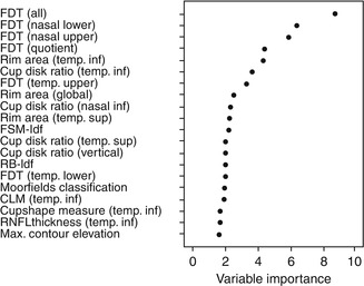
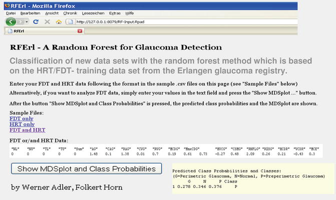
Fig. 3.2
Twenty most important variables of both diagnostic instruments ranked by the prediction accuracy for giving the correct classification. The variable importance measure was determined by the random forest method using the data of the learning data set. FSM-ldf, RB-ldf built-in classifiers using linear discriminant functions, CLM contour line modulation, RNFL retinal nerve fiber layer, temp temporal, inf inferior, sup superior, FDT frequency doubling technology
Fig. 3.3


An Internet browser tool was developed for the classification of new data sets from FDT perimetry and/or HRT. HRT Heidelberg Retina Tomograph, FDT frequency doubling technology. This platform includes all information of our learning cohort and can be easily installed on every computer. It generates the predicted class probability (yellow field) and an MDS (multidimensional scaling) plot for new data
Stay updated, free articles. Join our Telegram channel
Full access? Get Clinical Tree
