The results are shown in Fig. 3.1.
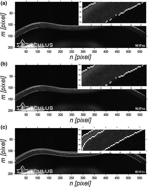

Fig. 3.1
Images L DSG , L DPG , L DCG and their zooms in the range m ∈ (1, 65), n ∈ (125, 146) obtained from the image L G by converting pixels to white in places where edges were detected, images a L DS , b L DP , c L DC respectively
The presented results show that the Canny edge detector is the best. Unfortunately, even this type of detector has drawbacks which include:
lack of edge continuity,
a significant amount of noise in the form of isolated white pixels as well as pixels forming small groups—several, several dozen,
no possibility of medical interpretation of detected edges.
For these reasons, especially the last one, new corneal edge detection methods will be proposed.
3.2 The First New Edge Detection Method
The need to propose new, dedicated, corneal edge detection methods is due mainly to the need to ensure its continuity and diagnostic interpretation. In this case, the discussed method was initially limited to the detection of the outer corneal edge. At the outset, it can be assumed that for each column of the image L G (m, n) there is at most one point of the outer corneal edge L d (n). In the absence of the corneal contour, the obtained values will be equal to M. After a rough analysis of the results obtained during image pre-processing, it turned out that one of the methods that can provide satisfactory results is looking for the greatest gradient in relation to specific points of the selected column in the image L G , L MED or L O . For example, for the image L G it will be L dG (n) equal to:


(3.1)
m ∈ (1, M − 1).
If there is more than one identical maximum value, only the first one in the order in which the rows are analysed is taken into account. This is due to the position of the cornea which is the first object when looking at the image L G from the top. At this point, I encourage readers to test the following source code fragment (after having loaded the image L G ):

The proposed method has its drawbacks. The main ones are high sensitivity to noise and brighter objects that occur in the depth of the eye, for example, parts of the iris which are often visible. A similar situation takes place after the removal of uneven background or histogram equalization. Therefore, it is necessary to carry out additional methods which will later allow for unambiguous determination of the outer corneal contour. These methods include morphological methods, in particular, erosion and dilation. In the case of a symmetrical structural element SE 2 , a new image L C will be determined after a close operation with the following formula:


(3.2)
An important element is the size of the structural element SE 2 . This size has been tested in the range from M SE2 × N SE2 = 3 × 3 pixels to M SE2 × N SE2 = 13 × 13 pixels. This will be further a parameter set by the application user. The next step, directly related to morphological opening, is automatic histogram analysis—L HIST . The designated histogram is subjected to careful analysis. For the counted number of pixels, for example, for the image L MED :


where L HIST (p r2 ) contains a number of brightness pixels equal to the value p r2 . In the next step, the binary image L BIN1 is obtained, i.e.:

where p r3 is the threshold selected once during the analysis, p r3 ∈ (2, 20). These relationships can be easily written as a code in the following form:

(3.3)

(3.4)

(3.5)

The above code includes new functions such as: hist designed to calculate the histogram for brightness values in the range (0.255), and bar and line associated with the GUI and providing a bar graph and a line. In the above code, the value p r3 was changed in the range p r3 ∈ (2, 7, 12, 17). The results obtained for i = 72 and p r3 = 2 as well as p r3 = 7 are shown in Fig. 3.2.
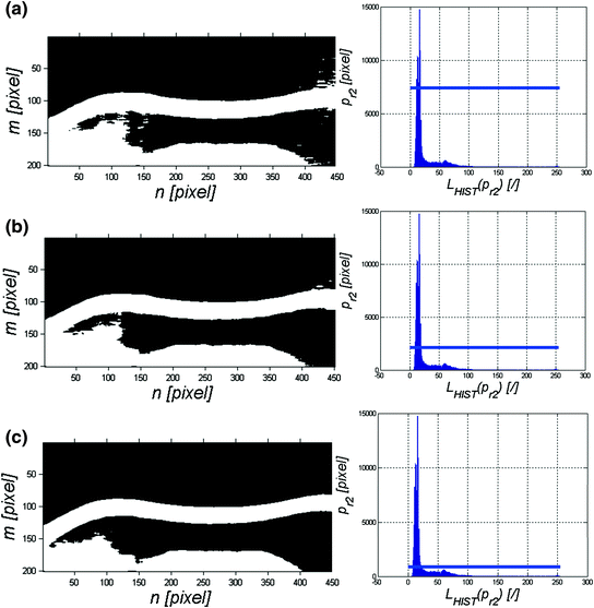

Fig. 3.2
Image L BIN and histogram of the image L MED for i = 72 and p r3 = 2 (a); p r3 = 7 (b) and p r3 = 17 (c). Additionally, the histogram graphs show in blue the cut-off line, the thresholding line
The images L BIN shown in Fig. 3.2 enable, at this stage, to determine the correct position of the outer corneal contour. However, the fact that the cornea is the largest object on the scene allows for the use of another operation—labelling. Labelling enables to replace the successive values of clusters in the binary image with their labels. The function bwlabel is designed for this purpose. Assuming that two vectors, the label and the area corresponding to its cluster, will be stored in the variable pam, this fragment of the source code can be written as:

This method is applicable in all situations for which the object of interest is the largest of all objects and there is a significant amount of noise. As shown in Fig. 3.3, all isolated small objects visible on the right side of the image have been removed. Unfortunately, the shape of the largest object, the cornea, remains unchanged after this operation. In this case, distortions of the outer corneal contour are visible—mainly in the right part of the image (Fig. 3.3).
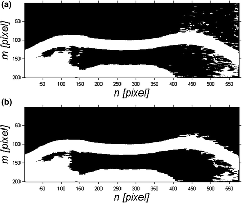

Fig. 3.3
Image L BIN (a), and binary image L BIN2 (b) with only the largest object left
However, the binary image L BIN2 , owing to the automatic adjustment of the binarization threshold (Fig. 3.2), provides correct analysis results. Using a simple method for finding the first value equal to one in each column of the image, it is possible to find the waveform of the outer contour L dBIN2 (n) with no significant obstacles:

for L BIN2 (m, n) = 1.

(3.6)
This method, used for i images, enables to obtain a three-dimensional image, the outer surface, the reaction of the eyeball to an air puff—the waveform L E (n, i)—Fig. 3.4.
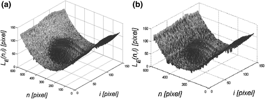


Fig. 3.4
Image L E (n, i) obtained for a p r3 = 10 and b p r3 = 2
< div class='tao-gold-member'>
Only gold members can continue reading. Log In or Register to continue
Stay updated, free articles. Join our Telegram channel

Full access? Get Clinical Tree


