Visual Acuity in the Young Child
Robert H. Duckman
Ask the question: “Why does the clinician measure visual acuity in the adult?” The answer would be that, in the adult, visual acuity is a relatively simple and reliable clinical finding that should be a good indication of that person’s visual function. If visual acuity were diminished, the clinician would take that finding as a sign that some interruption had occurred to normal acuity (e.g., refractive error, cataracts, retinal disease, or other ocular pathology). It could also indicate a dysfunction of ocular motility (e.g., nystagmus or eccentric fixation), central nervous system disease, and so forth. Ocular disease and visual acuity are usually highly correlated with one notable exception—glaucoma. Visual acuity is the foremost single test used to describe visual function of a human being. In the adult population, it determines whether people can qualify for a license to drive a car or fly a plane, be a police officer, or serve in the armed forces. It may not be the best gauge of a person’s visual function, but visual acuity is surely the easiest and fastest means of determining if a person’s visual function is in tact. This may not, however, be the case with infants. A series of developmental processes must occur before visual acuity can be considered to be 20/20. It has been demonstrated that infants under the age of 48 weeks post-conceptional age (PCA) with compromised visual cortices can demonstrate normal visual behaviors (1). In addition, the acquisition of visual acuity data is done by different methodologies than it is in the adult; therefore, although it gives us data, it may not necessarily be comparable data, regarding visual acuity.
Clinically, the visual acuity finding is used to “guide” us through the examination. That is, if visual acuity is normal (Snellen VA 20/20), the clinician can infer that little refractive error exists, probably the macula areas are healthy, and no pathology is present that compromises the acuity of the person. Can the clinician make the same assumptions when measuring the infant’s visual acuity? Not necessarily. Visual acuity development in the human infant follows the “law of improvement” (i.e., developmentally, the visual acuity starts out poorly and, over time, gets better). Much of the improvement results from anatomic and physiologic changes that occur in normal development (see Chapter 1). Decreased visual acuity in the infant, thus, does not give the clinician the same assurance that visual function is in some way disrupted. Rather, it must be considered within a developmental time table and the status of the infant during testing. If a testing procedure demands attention and the child is not sufficiently attentive, visual acuity values would be lower than they would be if the child were fully attentive.
Subsequent visits, with the child in a more “cooperative” state, could yield more accurate and better acuity values. If during the examination the child is inattentive and uncooperative, it is often necessary to reschedule the child for another appointment.
Also, again remember that, depending on the child’s age and the measuring instrument, it is normal to find infant acuity to be lower than that of an adult. In the evaluation of infant visual acuity, it is expected and common to find lower acuity values in the absence of any significant clinical findings. Then, with growth and maturation, the test results will approach adult levels of acuity, but at different times for different techniques and different individuals.
The infant is born with expected and normal lowered visual acuity. Visual acuity is expected to improve over the course of time. This chapter examines this development and how it proceeds. Normative data are important if we want to make any statement about an individual child’s visual function. In the pediatric population, any visual acuity measurement must be considered within the context of two pieces of information:
What methodology was used to measure the visual acuity?
How old is the child?
For example, if an infant is shown to have 20/100 visual acuity, we cannot know if this is a normal finding or an abnormal finding until we have answered the two questions. If the child is 8 months old and the measurement is done with visual evoked potentials (VEP), the finding would be abnormal because the infant 6-months of age should be able to respond to checkerboard squares equivalent to 20/20 on a VEP. If, however, the child is 6 months old and the methodology used is forced choice preferential looking, this would be an expected and normal acuity value for the child at this age.
Before discussing the development of visual acuity, it is important to define the different types of visual acuities that can be measured. Basically, four types of acuity measurement are used, which will be discussed. Each is different and comparison between types may be inappropriate. For example, if a child has a spatial acuity of 30 cycles per degree (spatial separation equivalent to 20/20 acuity) and another child has a recognition acuity of 20/20, they should not be compared as if equivalent. They are not!
The four types of visual acuity that are generally considered are:
Minimum visible or detection acuity is being able to tell that a given visual stimulus is present or not, or what is the smallest stimulus an individual can detect. Detection acuity is not the best descriptor of visual acuity because it is stimulus bound (i.e., by changing the strength of the stimulus you can alter the visual acuity value). If, for example, you take a very small opening in an otherwise opaque background and put a light stimulus behind the hole and the person may or may not see it. If, however, the person does not see it, and you can increase illumination until the individual is able to tell that it is there, you will have changed the acuity by changing the stimulus. If modulating the stimulus can change the acuity, it may be an inaccurate way to quantify acuity.
Minimum separable or resolution acuity is a measure of a person’s ability to detect separation of contours. The smaller the separation of the acuity prototype elements that the person can resolve, the better the resolution acuity (Fig. 2.1).
Teller acuity cards (TAC) present square wave spatial frequency gratings on a gray background matched for mean luminance in a forced choice preferential looking (FPL) paradigm. The patient will be attracted to the striped stimulus as long as the contours between the black and white stripes can be seen. Once the width of the stripes falls below the child’s threshold to resolve the detail, the infant will no longer be able to perceive the square wave gratings as a striped field. It will blend into a gray field that has been matched to the mean luminance of the gray background. Now, instead of seeing a striped stimulus on a gray background, the child will see a gray stimulus on a gray background. Once this happens, the preference the child had previously demonstrated for the striped stimulus, disappears. As long as the child is capable of resolving the stimulus detail and is attending to the task, the preference will be noted. The highest spatial frequency (narrowest
line width) that produces a positive preference response will be the minimal separable visual acuity or spatial acuity. As with other types of acuity measures, minimal separable acuity starts out poorly and improves over time. Although most discussions of minimal separable visual acuities equate them to Snellen acuity equivalents on the basis of angular subtense, the minimal separable acuity is not synonymous with recognition acuity (see below).
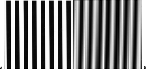
Figure 2.1. A: Spatial frequency square wave grating—higher spatial frequency. B: Spatial frequency square wave grating—lower spatial frequency.
Vernier acuity (hyperacuity) is a measure of the eye’s ability to perceive that a disalignment exists between the elements of the stimulus when compared with a stimulus without such disalignment. The eye has a better ability to perceive the disalignment than to be able to resolve adjacent contours (resolution acuity) by a factor that changes over time and from 3 months on surpasses resolution acuity (2,3,4). Therefore, this is often referred to as hyperacuity. Hyperacuity can be measured via an FPL type paradigm where the infant will show a preference for the disaligned square wave grating stimulus over the aligned stimulus as long as the disalignment can be perceived (Fig. 2.2).
Recognition acuity is the type of acuity measurement normally used clinically on patients who are old enough to subjectively report what they see on the typical Snellen acuity letter chart, pictures, numbers, and so forth. The age at which children can do this varies greatly, but starts at about 2 to 2.5 years of age. It involves being able to resolve the detail in the optotype and, on a cognitive level, to identify what the stimulus is. The differences between number or letter optotypes and pictures will be discussed in Chapter 10. Now, it is important to be aware that acuity values tend to be somewhat higher when picture optotypes are used than when letter or number optotypes are used. Recognition acuity, however, is the most universally used acuity measurement on patients who are old enough to respond to this type of testing.
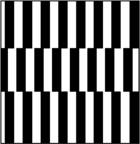 Figure 2.2. Vernier spatial frequency target. |
Visual acuity values in infancy and early childhood are reflective of the acuity technique being used, the critical immaturities of the visual system (see Chapter 1), the child’s developmental status, cognitive awareness, and attention to the visual input.
For decades clinicians and researchers have looked at the development of visual acuity. During that time, the base of knowledge has changed significantly because of increased understanding of visual development and the increasing sophistication of the experimental paradigms being used to measure function. Before the vision scientist can look at the development of visual acuity, an instrument or instruments must be available to measure that function. The development of these instruments started in the laboratory and, as soon as practicable, spread throughout the clinical community.
Teller and Movshon (4) described the “ancient history” of visual development as the early 1960s. And if you examine the work on visual development before the 1960s, “you will not have far to travel.” It is sparse and often the results are questionable. For example, before this time, the only real work on visual acuity in infants used optokinetic nystagmus (OKN) as the measuring tool. Aside from being a difficult observation to make in infants (observers often filmed a baby’s eyes during the presentations so they could go back afterward to study whether the OKN was present), it has been shown that infants with considerable loss or total absence of visual cortex can demonstrate OKN (5,6,7). Daw (8) reported that “OKN is believed to be primarily a subcortical phenomenon, and needs a stimulus covering a substantial amount of the visual field.” For an observer to elicit the OKN response, a child must attend to the drum and accommodate to its surface. The absence of a response might be nothing more than inattention. Thus, we are unable to draw definitive conclusions from either its presence or its absence.
In the early 1960s, Fantz (9,10,11) published his results of looking at an infant’s pattern preferences using a procedure called “preferential looking” (PL). By 1962, Fantz et al. (12) published data on the early development of visual acuity by use of his PL technique and compared it with OKN responses by the same infants. The acuity values that Fantz reported, at that time, closely reflect acuity values currently accepted for infants’ spatial vision.
As recently as the early 1970s, if parents asked a pediatrician or eye care professional what their baby’s vision was, the typical response would be something like “We will have to wait until around 5 years to know for sure. However, your baby fixes and follows” (meaning that the child could fixate and track a trans-illuminator or other visual stimulus). Indeed, many continue to evaluate an infant’s early visual function on the basis of the “fix and follow” response. An ever increasing number of clinicians, however, attempt to quantify, either electrophysiologically or behaviorally, the visual acuity of the infant or toddler patient. This turning point for clinical evaluation of infants’ visual acuity resulted from the work that Fantz published in the 1950s, 1960s, and 1970’s. Fantz (13) noticed that infants had definite preferences when it came to looking at objects. His work clearly showed that these preferences were the natural predilection of the healthy, normal human infant. Infants, when given a choice, will show definite behavioral differences and prefer to look at objects with higher contrast, greater number of contours, and greater complexity over more simple patterns or homogenous backgrounds (13). In 1975, Fantz and Fagan (14) published findings showing that during the first 6 months of life, infants differentially prefer to look at objects of greater complexity over objects of simpler design. Later that same year, Fantz and Miranda (15) found that neonates show a differential preference for curved lines over straight lines. The other issue of interest is that these predilections were directly related to PCA and not chronological age. Fantz did an enormous amount of “observing” of infant visual behavior, and the message is that, given the choice to fixate a patterned field over an unpatterned, homogenous field matched for mean luminance, the infant will look at the patterned field. This is the basic premise of what has become the most utilized behavioral, clinical technique to evaluate visual function in infants today—forced choice preferential looking.
Forced choice preferential looking has evolved over approximately the past 35 years. It uses the premise that infants prefer to fixate
“something” over nothing at all. When the “something” is a spatial frequency grating, the assumption is that if spatial frequency is paired with a homogenous gray field of matched luminance, as long as the child can resolve the stripes as stripes, the infant will prefer to fixate that target. When the spatial frequency falls below threshold and the infant’s ability to resolve detail has been surpassed, the stripes will now appear gray and the preference previously seen for the pattern disappears.
“something” over nothing at all. When the “something” is a spatial frequency grating, the assumption is that if spatial frequency is paired with a homogenous gray field of matched luminance, as long as the child can resolve the stripes as stripes, the infant will prefer to fixate that target. When the spatial frequency falls below threshold and the infant’s ability to resolve detail has been surpassed, the stripes will now appear gray and the preference previously seen for the pattern disappears.
The typical stimulus for FPL has almost always been square wave spatial frequency gratings. Spatial frequency gratings are described by the number of cycles (one black stripe and one white stripe per cycle) they subtend at the eye per degree of visual angle. The lower the number of cycles, the fewer the number of black and white stripes per degree of visual angle. The greater the number of cycles per degree of visual angle, the greater the number of stripes. Thus, high spatial frequencies are finer black and white lines than lower spatial frequencies lines, which are wider. A spatial frequency that is easy to remember is the spatial frequency of 30 cycles per degree (cpd). Thirty cycles per degree is equivalent to the resolution necessary to see 20/20 optotypes. It is unclear whether these acuity values are equivalent and they probably are not. In any case, it is not appropriate to express spatial acuity in Snellen equivalence (although it is done all the time), but rather they should be expressed in cpd.
From the early 1980s through the present time, much data has been collected assessing the visual acuity of infants by behavioral and electrophysiological procedures.
While researching material for this chapter and to offer an idea of the growth in interest in the area of infant vision, a search from 1960 to 1970 on infant visual acuity produced citations of just over one page (15). The same topic sampled from 1970 to 1980 produced 17 pages of citations (244).
Forced Choice Preferential Looking
As early as 1978, Dobson et al. (16) were exploring the utilization of the innate response of the infant to preferentially fixate a pattern over nothing at all in a behavioral paradigm to quantify “visual acuity,” perhaps the beginning of FPL as a clinical tool. Before this, however, significant data were collected by psychometric means to establish the norms for this type of “acuity” measurement. In the psychometric procedure, the researchers would take all their spatial frequency slides, match them up with slides of equal luminance and randomly place all of them in pairs for presentation to the infants. Two people were required to run the paradigm—one to make the presentations to the infant and the “blind” observer who would watch to see where the child looked. The person controlling the presentations would record whether the “blind” observer was correct or incorrect. After all presentations were made, the psychometrists would go back and score the responses to see at which spatial frequency value the observer (infant) fell below 75% criterion level for correct responses. For example, if a child “saw” three quarters of the presentations at 4.9 cpd, but only half of the presentations at 6.5 cpd, then that child’s threshold visual acuity would be 4.9 cpd. This paradigm involved a minimum of two people, sufficient time to make more than 100 presentations and a cooperative, attentive infant throughout the testing. Psychometric measurement could never be used clinically because it took too long, often requiring multiple visits to define threshold acuity. This was not a tenable clinical tool. It was an extremely difficult research procedure as well. In an attempt to make the FPL procedure easier and less time consuming, change came in the form of procedural “short cuts” (17,18,19,20,21).
In an attempt to streamline the procedure, Dobson et al. (22) attempted to define the “diagnostic stripe widths” (DSW) for infants at different ages. They wanted to find the age norms for FPL and what should be expected of a child by a certain age. Dobson et al. (22) obtained what they called “a preliminary estimate of the DSW.” The study had a sample of 76 normal infants, of whom 69 infants (91%) completed testing. Dobson acknowledged that normative data would require a larger sample. The success with which the data were collected confirmed ages at which visual acuity levels should be attained. Dobson et al. defined the DSW as “the minimum stripe width to which infants with normal
visual acuity will readily respond” at a given age. They evaluated children 4, 8, 12, and 16 weeks of age to find the minimal stripe width to which each age group would respond. This was one of the earliest attempts to take FPL out of the laboratory and into clinical use. With known values of what an infant should respond to by a given age, a clinician would be able to tell whether visual acuity for any child was normal for age. It would not provide a visual acuity threshold. The idea was that with norms for given ages, the clinician would take spatial frequency gratings of that child’s diagnostic stripe width, show them a set of spatial frequency slides with their matched grays, and see whether the blind observer was correct 70% to 75% of the time. If so, the clinician could say that visual acuity development was normal for this child. The clinician would not know whether the infant could see better than his or her DSW, but would know that this child was where he or she was supposed to be for normal vision development. It was a much more practical thing to do clinically. In time, the following DSW were determined and utilized in the DSW procedure: The age norms for FPL DSW procedure are discussed below with the approximate Snellen equivalents (Table 2.1).
visual acuity will readily respond” at a given age. They evaluated children 4, 8, 12, and 16 weeks of age to find the minimal stripe width to which each age group would respond. This was one of the earliest attempts to take FPL out of the laboratory and into clinical use. With known values of what an infant should respond to by a given age, a clinician would be able to tell whether visual acuity for any child was normal for age. It would not provide a visual acuity threshold. The idea was that with norms for given ages, the clinician would take spatial frequency gratings of that child’s diagnostic stripe width, show them a set of spatial frequency slides with their matched grays, and see whether the blind observer was correct 70% to 75% of the time. If so, the clinician could say that visual acuity development was normal for this child. The clinician would not know whether the infant could see better than his or her DSW, but would know that this child was where he or she was supposed to be for normal vision development. It was a much more practical thing to do clinically. In time, the following DSW were determined and utilized in the DSW procedure: The age norms for FPL DSW procedure are discussed below with the approximate Snellen equivalents (Table 2.1).
Dobson (21) discussed the slowness of behavioral techniques from the laboratory entering the clinical arena. She observed that OKN “is used widely by ophthalmologists as an informal, subjective estimate of an infant’s visual status.” The shortcomings of the OKN response limits it in the amount of information it can provide. On the other hand, the emergence of the FPL procedures, in the form of the diagnostic stripe width procedure, that had only recently been introduced into clinical settings, promised a lot more. Dobson further observed that the procedure “appears to be effective in diagnosing infants with ophthalmic problems that would be expected to interfere with vision tested binocularly.”
Table 2.1 Diagnostic Stripe Width from 1–9 Months | ||||||||||||||||||
|---|---|---|---|---|---|---|---|---|---|---|---|---|---|---|---|---|---|---|
|
About the same time, Gwiazda et al. (23,24) started using their “fast” PL procedure to collect data on normal infants during the first year of life. Their babies ranged in age from 2 to 58 weeks of age. In the healthy, normal infant without visual problems, their technique measured visual acuity in less than 5 minutes—a vast improvement over the psychometric procedures discussed earlier. Although the data they were trying to gather replicated earlier experiments, the earlier data were collected with a much lengthier paradigm—the 60-trial method of constant stimuli. They were looking to see if the faster method produced similar results. They used gratings ranging from 1.5 to 18 cpd in approximately half octave steps. They measured acuity for horizontal, vertical, and right oblique gratings. They found that a steady increase in acuity occurred from 4 weeks to 1 year of age. Acuity for horizontal and vertical spatial frequency gratings increased from 20/1200 at 4 weeks to 20/50 for horizontal and 20/60 for vertical at 1 year of age.
In 1982, Mayer et al. (25) used a staircase PL presentation to evaluate visual acuity in children aged 11 days to 5 years, known to have an ophthalmologic disorder. In the psychometric PL measurement of acuity in infants, it was necessary to take all the spatial frequency slides with their matched grays, randomly present them in pairs, and go through all the stimuli before going back to see where the responses fell below the criterion level of 70%. With the staircase presentation, the stimuli were presented in pairs, except the pairs were ordered from lowest spatial frequency (widest stripes) to highest spatial frequency (thinnest stripes). The experimenter would then start at the beginning of “the staircase” (lowest spatial frequency) with stimulus pairs, and continue presenting them until the child stopped showing a preference for a stimulus 70% of the time. At that point, the experimenter would have a threshold visual acuity, and no trials would be given beyond that threshold level. This significantly decreased the amount of time for both testing and scoring these patients.
Mayer et al. (25) noted that “acuity of infants and young children with normal eyes, obtained by the PL staircase procedure” agreed well with acuities obtained previously by the method of constant stimuli. This was a good indication that the faster methodology would yield visual acuities as accurate as the longer one.
Mayer et al. (25) noted that “acuity of infants and young children with normal eyes, obtained by the PL staircase procedure” agreed well with acuities obtained previously by the method of constant stimuli. This was a good indication that the faster methodology would yield visual acuities as accurate as the longer one.
Stay updated, free articles. Join our Telegram channel

Full access? Get Clinical Tree


