Purpose
To assess between- and within-individual variability of macular cone topography in the eyes of young adults.
Design
Observational case series.
Methods
Cone photoreceptors in 40 eyes of 20 subjects aged 19–29 years with normal maculae were imaged using a research adaptive optics scanning laser ophthalmoscope. Refractive errors ranged from −3.0 diopters (D) to 0.63 D and differed by <0.50 D in fellow eyes. Cone density was assessed on a 2-dimensional sampling grid over the central 2.4 mm × 2.4 mm. Between-individual variability was evaluated by coefficient of variation (COV). Within-individual variability was quantified by maximum difference and root mean square (RMS). Cones were cumulated over increasing eccentricity.
Results
Peak densities of foveal cones are 168 162 ± 23 529 cones/mm 2 (mean ± SD) (COV = 0.14). The number of cones within the cone-dominated foveola (0.8–0.9 mm diameter) is 38 311 ± 2319 (COV = 0.06). The RMS cone density difference between fellow eyes is 6.78%, and the maximum difference is 23.6%. Mixed-model statistical analysis found no difference in the association between eccentricity and cone density in the superior/nasal ( P = .8503), superior/temporal ( P = .1551), inferior/nasal ( P = .8609), and inferior/temporal ( P = .6662) quadrants of fellow eyes.
Conclusions
New instrumentation imaged the smallest foveal cones, thus allowing accurate assignment of foveal centers and assessment of variability in macular cone density in a large sample of eyes. Though cone densities vary significantly in the fovea, the total numbers of foveolar cones are very similar both between and within subjects. Thus, the total number of foveolar cones may be an important measure of cone degeneration and loss.
Macular cone photoreceptors in the human eye are responsible for high-acuity vision and color vision. The spatial density of cone photoreceptors (cells/mm 2 ) is an essential metric for assessing the fundamental limit of human vision and the effect of aging and disease. To ensure the validity of spatial density, accurate knowledge of cone topography and variability in adults in normal chorioretinal health is of paramount importance.
In 1990, Curcio and associates presented a comprehensive 2-dimensional map of both cone and rod density in 7 short–post mortem retinas prepared as whole mounts. This technique enabled visualization, topography, and morphologic detail of inner segments, while largely eliminating histologic processing artifacts and counting errors due to cells split by sectioning. This widely cited study quantified salient features of human cone topography hinted in previous studies examining small retinal areas. These features include a peak of cone density at the foveal center, a sharp decline from the center, a lesser decline with increasing eccentricity, isodensity contours elongated along the horizontal meridian, and higher density in nasal than temporal periphery. With accurately localized foveal centers, it was possible to compare within- and between-individual variability in cone density and find a striking (3-fold) range of peak cone density. A subsequent study by the same authors showed that despite this wide range in density, the total number of cones within the 0.8 to 0.9 mm diameter cone-dominated foveola was much less variable. Photoreceptor distributions in 1 pair of fellow eyes were similar but not identical, with an 8% difference in cone number and density differences up to 30% in spots.
Recent advance in adaptive optics (AO) assisted retinal imaging has made it possible to assess in the living human eye cone density, which could be characterized previously only by histology. Although AO retinal imaging offers significant advantages in studying the impact of chorioretinal diseases on cones, the density and the variability of the foveal cones, especially cones in the very foveal center, have not been adequately assessed. Paucity of these data may impede use of this imaging modality for larger studies involving more individuals. Recent technical progress in adaptive optics scanning laser ophthalmoscopy (AOSLO), including a new-generation AOSLO that is used herein, has provided appropriate resolution for imaging foveal cones. The goal of this study is to better assess between- and within-individual variability of cone topography in a large number of young adult subjects and to determine the total number of foveolar cones. Many of the same advances originally developed for accurate histology are now possible with in vivo imaging.
Methods
The study followed the tenets of the Declaration of Helsinki and was approved by the Institutional Review Board at the University of Alabama at Birmingham. Written informed consent was obtained from participants after the nature and possible consequences of the study were explained. The study complied with the Health Insurance Portability and Accountability Act of 1996.
Subjects
Twenty subjects between 19 and 29 years of age were recruited from the student and employee population at the University of Alabama at Birmingham (UAB). After written consent was obtained, a self-report questionnaire was administered to assess participant general health and ensure that only subjects in good chorioretinal health and free from systemic diseases were included. We excluded the subjects who had undergone any keratorefractive procedures such as laser-assisted in situ keratomileusis, which could influence the accuracy of the retinal magnification factor. Then, participants underwent assessment of best-corrected visual acuity (BCVA) using the Electronic Visual Acuity (EVA) tester and measurement of refractive error using an automated refractor. Eye lengths were measured using an ocular biometer (IOLMaster 500; Carl Zeiss Meditec, Dublin, California, USA). To minimize the effect of refractive error, only participants with refractive error between −3 diopters (D) and 0.625 D and fellow eye refractive error difference <0.50 D were included.
Adaptive Optics Scanning Laser Ophthalmoscopy Imaging
Both eyes of subjects were imaged with the UAB AOSLO. Specifications have been reported elsewhere. In brief, the light source is a superluminescent diode (SLD) (Broadlighter S840-HP; Superlum, Moscow, Russia). The wavelength is centered at 840 nm with a spectral bandwidth of 50 nm. This low-coherence light source produces high-fidelity retinal images by reducing light interference. The pupil size of the instrument is set at 6 mm diameter for young subjects. The AO consists of a deformable mirror with 97 actuators (Hi-Speed DM97-15; ALPAO SAS, Montbonnot, France) and a custom high-speed wavefront sensor. The robust performance of the AO ensured that all cone photoreceptors were resolved across the maculae in all eyes. The imaging light power measured at the cornea was 500 μW, or 3.8% of the maximum exposure permitted by the ANSI standard. The AOSLO imaging channel consists of a photomultiplier tube (PMT) (H7422-50; Hamamatsu Photonics K.K., Hamamatsu, Shizuoka, Japan) and custom signal processing electronics controlling the scanning system and forming the output of the PMT to a video signal. The AOSLO acquires retinal images with a frame rate of 15 Hz. The field of view subtends approximately 1 degree × 1 degree and the image is recorded at 512 × 512 pixels/frame.
The subject’s pupil was dilated with 1.0% tropicamide and 2.5% phenylephrine hydrochloride. The head was aligned and stabilized with a head mount and chinrest. A fixation target consisting of a moving light dot on a calibrated grid was placed in front of the eye via a pellicle beam splitter. At each point on the grid, the light dot paused for 2–3 seconds so that at least 30 frames were acquired. The subject was asked to follow and focus on the light target, while the AOSLO continuously recorded video across an area of 10 degrees × 10 degrees in the central macula. The continuously recorded retinal video allows a large macular image to be montaged from a series of successive frames with precise cone-for-cone registration in the overlapping area. A typical imaging session for both eyes lasted approximated 40 minutes.
Image Processing
Image distortion caused by nonlinear scanning by the resonant scanner and by eye movements was eliminated by custom software. Registered images (typically 10–30 frames) were averaged to enhance the signal-to-noise ratio. Images from different retinal locations were manually aligned (Photoshop; Adobe Systems Inc, Mountain View, California, USA) to create a continuous montage. Alignment was done on a cone-for-cone basis in areas of overlap.
Retinal Magnification Factor
The angular pixel size of AOSLO images (degree/pixel) was computed using a calibrated grid placed at the retinal plane of a model eye. To convert angular scale to linear on the retinal plane, we used the distance from the imaging space nodal point to the retina to calculate individual retinal magnification ratios (retinal magnification factor; RMF). This distance was calculated with the Liou and Brennan eye model, which closely resembles the in vivo biological eye. Model parameters, including anterior radius of curvature of the cornea (r1), anterior chamber depth (ACD), and axial length, were measured from each subject’s eye with the IOLMaster. Corneal thickness was subtracted from the measured ACD to obtain the distance from the posterior cornea to the anterior lens. The posterior radius of curvature of the cornea (r2) was estimated by 0.8236 × r1. The distance from the nodal point to the retina, N L , was calculated with optical design software (Zemax EE; Radiant Zemax, Redmond, Washington, USA). RMF was obtained with the equation RMF = N L tan1 o .
Cone Density Measurement
Accurate quantification of macular cone distribution and variability has several technical challenges. First, the singular point of high density (ie, the foveal center) must be accurately localized to serve as the origin of a coordinate system. Second, the steep gradient of cone density dictates the use of closely spaced sample points to avoid interpolation artifacts. Third, it demands the use of appropriately sized sampling windows to avoid artificial dilution of cone density at the peak. Fourth, even with robust AO correction for the wave aberration of the eye, visibility of cones in the foveal center may still be affected by light interference. To meet these demands, we sampled at closely spaced points in the fovea where the cone density gradient is steep, optimized window size to capture the maximum density within the foveal singularity, and pooled data from small windows enclosing well-visualized cones to use all possible data in the foveal center.
Retinal Coordinate System
The location of peak cone density served as the origin of a coordinate system with the abscissa along the temporal-nasal direction and ordinate along the inferior-superior direction. Based on the individual RMF, we generated a fiducial grid to mark the locations of sampling windows ( Figure 1 ). We put a 40 μm × 40 μm window over the area with the highest apparent cone density and then put 5 small windows of 5 μm × 5 μm size within this large window. We pooled cones in the 5 small windows to obtain an average and adjusted the position of the large window to set the origin of the retina coordinate.
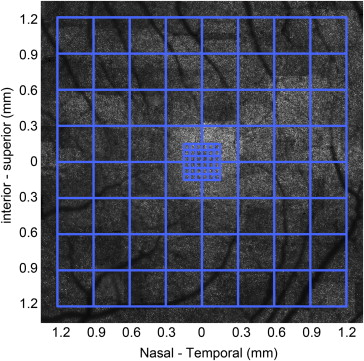
Sampling Strategy
The sampling pattern was adapted from that used in the histologic study, where it was determined empirically to produce smooth isodensity contour maps, even near the foveal singularity. As shown in Figure 1 , cone density was assessed at each intersection on this grid. At eccentricities ≤150 μm, the sampling interval is 50 μm; between 300 and 1200 μm eccentricities, the interval was 300 μm. In the fovea (0–150 μm eccentricity), sample windows were pooled, as described above. To avoid blood vessels and seams in the image montage, sampling window positions were slightly adjusted.
Optimal Sampling Window
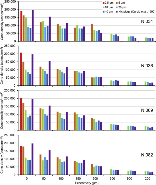
We assessed cone densities with different-size square sampling windows (2.5–40 μm on a side) in the eyes of 4 subjects ( Figure 2 ). The windows were selected based on center-center spacing provided by histology ; for example, at the foveal center, where cone spacing is 2.4 μm, we tested the cone density measurement using square windows of sizes from 2.5 μm to 40 μm. The 2.5 μm window encompassed a single cone; thus it was used for ascertaining that no cone-like spot with size bigger than 2.5 μm could be taken as cones. At ≥50 μm eccentricity, where cone spacing is >2.7 μm, square windows of 5–40 μm were tested. Through this process, we determined a series of heuristically optimal windows that yielded both a monotonically decreasing cone density profile with increasing eccentricity and cone densities close to the histologic reference data ( Table 1 ).
| Eccentricity | Optimal Window Size |
|---|---|
| 0–100 μm | 5 μm × 5 μm |
| 150 μm | 10 μm × 10 μm |
| 300–1200 μm | 40 μm × 40 μm |
Cone Counting
Based on the test in 4 subjects ( Figure 2 ), cone densities in the eyes of the rest of subjects (n = 16) were assessed with the optimal window at each eccentricity ( Table 1 ). To count cones automatically, we used the “find maxima” function of ImageJ (version 1.47g; http://rsbweb.nih.gov/ij/ ), with manual checking. A well-established practice to provide unbiased densities is to count cells only on the top and left edges of sampling windows, excluding those on the bottom and right edges. However, we adopted an alternative method. Using the ImageJ “find maxima” function, we counted cones including and excluding cells on the edges and then averaged the 2 measurements. Results obtained with these 2 methods in 4 subjects at the sampling points along the primary horizontal and vertical retinal medians differed by <3%.
Inter-rater reproducibility was assessed by the intraclass correlation coefficient (ICC) based on cone densities of 10 subjects measured by authors T.Z., P.G., and E.R.B. working independently. ICCs from the Shrout-Fleiss reliability random set were assessed along nasal-temporal and inferior-superior meridians. ICCs among 3 raters were greater than 0.99.
Quantitative Analysis and Statistical Evaluation
We computed mean density, standard deviation (SD), coefficient of variation (COV), and the total number of cones cumulated within rings of increasing eccentricity. We compared fellow eyes as follows:
- (1)
Maximum relative cone density difference: Relative cone density difference Δ i at each sampling point is estimated by (D OS − D OD )/D OD , where D OS and D OD are cone densities in the left and right eye, respectively.
- (2)
Root mean square (RMS) of the relative cone density difference at the individual sampling locations, which is calculated by RMSk=√∑i=Ni=1Δ2i/N
R M S k = ∑ i = 1 i = N Δ i 2 / N
, N is the number of subjects.
- (3)
RMS of the overall relative cone density difference across the studied retinal area, which is calculated by RMS=√∑k=Mk=1RMS2k/M
R M S = ∑ k = 1 k = M R M S k 2 / M
, M is the number of sampling points.
Within-individual variability was evaluated statistically using a mixed-model approach. The retina was divided into 4 quadrants: superior/temporal (S/T), superior/nasal (S/N), inferior/temporal (I/T), and inferior/nasal (I/N). The density within each quadrant was compared between fellow eyes, and a 3-way interaction term was included to examine whether the association varied across quadrants. The null hypothesis was that the distributions of fellow eyes of the same individual did not differ significantly. Analyses were performed using SAS v9.3 (SAS Institute Inc, Cary, North Carolina, USA). A P value < .05 was considered significant.
Stay updated, free articles. Join our Telegram channel

Full access? Get Clinical Tree


