Fig. 38.1
Schematic of the short-term sEPSM. The noisy speech (black) and the noise alone (grey) are processed separately through the model. The decision metric is based on the time-varying SNRenv
The running temporal output of each modulation filter is divided into short segments using rectangular windows with no overlap. The duration of the windows is specific for each modulation channel and is the inverse of the centre frequency of a given modulation filter (or the cut-off frequency in the case of the 1-Hz low-pass filter). For example, the window duration in the 4-Hz modulation channel is 250 ms. For each window, the AC-coupled envelope power (variance) of the noisy speech and the noise alone are calculated separately and normalized with the corresponding long-term DC power. The SNRenv of a window is estimated from the envelope power as

where P S+N and P N denote the envelope power of the noisy speech and the noise alone after the normalization. For each modulation channel, the running SNRenv values are averaged across time, thus assuming that all parts of a sentence contribute equally to intelligibility. The time-averaged SNRenv values from the different modulation filters are then combined across modulation filters and across gammatone filters, using the “integration model” from Green and Swets (1988). The combined SNRenv is converted to the probability of correctly recognizing the speech item using the concept of a statistically “ideal observer” (Jørgensen and Dau 2011).

(38.1)
3 Method
Model predictions were compared to data from the literature as well as data collected for the present study. The target speech was either Danish sentences from the DANTALE II speech material (Wagener et al. 2003), Danish sentences from the CLUE speech material (Nielsen and Dau 2009), or sentences from the TIMIT database. The data reflect either speech reception thresholds (SRTs) corresponding to the 50 % point on the psychometric function or percentage of correct scores. All subjects were normal-hearing listeners.
Three conditions of stationary interferers were considered: (1) speech-shaped noise (SSN), (2) car-cabin noise (CAR), and (3) the sound of bottles on a conveyer belt (BOTTLE). Moreover, three conditions with fluctuating interferers were considered: (1) a conversation between two people sitting in a café (CAFE), (2) SSN that was amplitude modulated by an 8-Hz sinusoid (SAM), and (3) the speech-like, but non-semantic, International Speech Test Signal (ISTS; Holube et al. 2010).
Finally, two conditions with nonlinear processing were considered: (1) speech mixed with SSN and further processed by spectral subtraction (Berouti et al. 1979) using six different values of the over-subtraction factor, ρ, and (2) clean speech distorted by phase jitter with a varying degree of the jitter constant, α (Elhilali et al. 2003).
For the predictions, the model parameters were calibrated to a close match between the predictions and the data for the unprocessed SSN condition for a given speech material. These parameters were then used for all other experimental conditions. Identical stimuli were used for the simulations as for obtaining the data, except for the conditions with phase jitter where the data were obtained using sentences from the TIMIT database (Elhilali et al. 2003), whereas the predictions were obtained using the CLUE sentences.
4 Results
4.1 Conditions with Stationary and Fluctuating Interferers
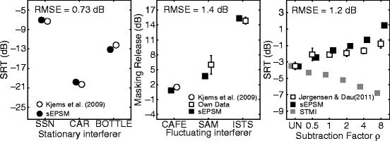
The left panel of Fig. 38.2 shows SRTs obtained by Kjems et al. (2009) (open circles) and corresponding predictions obtained with the sEPSM (filled circles) in the conditions with stationary interferers. The SRTs range from −17 to −7 dB, reflecting the differences of spectral masking for the various stationary interferers. The sEPSM accounts well for the SRTs for the three stationary conditions. The root mean square error (RMSE) between the measured and simulated data amounts to 0.71 dB.


Fig. 38.2
Measured (open symbols) and predicted (filled symbols) SRTs in conditions with stationary interferers (left panel), masking release in conditions with fluctuating interferers (middle panel), and SRTs in conditions with noisy speech processed by spectral subtraction
The middle panel of Fig. 38.2 shows the results for the fluctuating interferers, represented by the MR calculated as the difference between the SRT obtained in the SSN condition and a given condition with fluctuating noise. The MR is quite low for the CAFE noise compared to the other interferers, indicating that the fluctuations in this noise type are less useful for the listener. The greatest MR is found for the ISTS interferer. The sEPSM accounts for the MR effects obtained with the different interferers with an RMSE of 1.5 dB.
4.2 Conditions with Processed Noisy Speech
4.2.1 Spectral Subtraction
The right panel of Fig. 38.2 shows SRTs obtained by Jørgensen and Dau (2011; open squares) and corresponding predictions by the sEPSM (filled squares) for six conditions of ρ, where UN denotes the reference condition with no spectral subtraction. The data show an increase of the SRT with increasing ρ, demonstrating a lower intelligibility with spectral subtraction than without the processing. The sEPSM predicts the trends in the data, although it overestimates the SRTs for ρ = 2, 4, and 8 (RMSE = 1.2 dB). Predictions obtained with the STMI (grey squares) suggest that the intelligibility increases after spectral subtraction, in contrast to the measured data. The STMI thus fails to account for spectral subtraction, as does the STI (Jørgensen and Dau 2011).
Stay updated, free articles. Join our Telegram channel

Full access? Get Clinical Tree


