Introduction

Fig. 1.1

Image in the geometric coordinate system with points indicating brightness function domain pixels and squares representing detector sensors

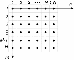
Fig. 1.2

Image in the screen coordinate system represented in the form of an array (m—row, n—column)

The order of giving the individual dimensions of the matrix (Fig. 1.2) was adopted in accordance with the nomenclature used in Matlab, FreeMat, Scilab or Octave. The first dimension is the row, the second dimension is the column and then there are other dimensions, wherein the numbering of these dimensions starts with one instead of zero. This is common numbering used in most of the publications devoted to image analysis and processing (Fig. 1.2). Thus, the specified coordinate system enables to define resolution as a pair of values M × N, where M is the number of rows of the image matrix and N is the number of columns, i.e.:

$L\left( {m,n} \right) = \left\{ {\begin{array}{*{20}l} {L\left( {1,1} \right)} \hfill & {L\left( {1,2} \right)} \hfill & \cdots \hfill & {L\left( {1,N - 1} \right)} \hfill & {L\left( {1,N} \right)} \hfill \\ {L\left( {2,1} \right)} \hfill & {L\left( {2,2} \right)} \hfill & \cdots \hfill & {L\left( {2,N - 1} \right)} \hfill & {L\left( {2,N} \right)} \hfill \\ \vdots \hfill & \vdots \hfill & {} \hfill & \vdots \hfill & \vdots \hfill \\ {L\left( {M - 1,1} \right)} \hfill & {L\left( {M - 1,2} \right)} \hfill & \cdots \hfill & {L\left( {M - 1,N - 1} \right)} \hfill & {L\left( {M - 1,N} \right)} \hfill \\ {L\left( {M,1} \right)} \hfill & {L\left( {M,2} \right)} \hfill & \cdots \hfill & {L\left( {M,N - 1} \right)} \hfill & {L\left( {M,N} \right)} \hfill \\ \end{array} } \right\}$

(1.1)

The image function L was defined as:

$L\left( {m,n} \right){:}\;C \times C \to C^{ + } \,\cup \, \left\{ 0 \right\}$

(1.2)

When the L function can take floating-point values, it can be written in the following way:

$L\left( {m,n} \right){:}\;C \times C \to R^{ + }\, \cup \,\left\{ 0 \right\}$

(1.3)

The individual function values are determined: on the set of integers (C ⁺ ∪ {0}) ∩ [0, q _w − 1], q _w ∈ C of quantization levels (generally q _w = 2⁸ = 256); or on the set of floating-point numbers, this is the range [0, 1]. Floating-point numbers are also written according to the nomenclature adopted in Matlab with dots as decimal separators. However, the individual elements (figures) are separated with a space or comma.

1.4.2 Contour and Edge

The contour in a monochrome 2D image is a line in the case of continuous structures or a group of pixels in the case of discrete structures. These are the points of the image function L, in the simplest case, with a constant brightness value. In the general case, they are directly linked with the object edges which are defined as physical, photometric and geometric points of the image function discontinuity. The edge is formed on the border of areas with different values of the image function L. The edge is the contour of the object. The most common and typical example of the edge including noise is shown in Fig. 1.3, where four cases are highlighted: (a) the ideal step profile, (b) the smoothed step profile, (c) the object with rising edges (d) the object with step edges.

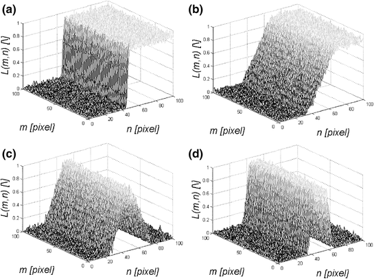
Fig. 1.3

Transverse profiles of the edges and objects in the image a the ideal step profile, b the smoothed step profile, c the object with rising edges d the object with step edges

Depending on the scale of consideration, the edges may also be classified as objects. This distinction is dependent on the definition of the object, and especially its minimum size.

1.4.3 Known Edge Detection Methods

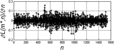
According to the afore-mentioned definition of the edge, it seems that the easiest way to detect it is to use differentiation operations. They provide information about brightness changes of the input image. For the sample image L(m, n) shown in Table 1.1, a profile of grey level changes L(m*, n) was formed, where m* is a constant value and in this case m* = 50 (see Fig. 1.3).

Table 1.1

Various stages of edge detection using information about the gradient

Symbol	Image/Graph
L(m*, n)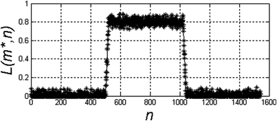
$\frac{{\partial \left( {L\left( {m^{*} ,n} \right)} \right)}}{\partial n}$

On this basis, it is possible to calculate:

$\frac{{\partial L\left( {m,n} \right)}}{\partial n} = \mathop {\lim }\limits_{{\Delta n \to 0}} \frac{{L\left( {m,n +\Delta n} \right) - L\left( {m,n} \right)}}{{\Delta n}}$

(1.4)

In the discrete case, it can be assumed that Δn is equal to one pixel, i.e. Δn = 1, and then:

$\frac{{\partial L\left( {m,n} \right)}}{\partial n}\,\hat{ = }\,\Delta _{n} = L\left( {m,n + 1} \right) - L\left( {m,n} \right)$

(1.5)

Similarly for the image axis m, i.e.:

$\frac{{\partial L\left( {m,n} \right)}}{\partial m}\,\hat{ = }\,\Delta _{m} = L\left( {m + 1,n} \right) - L\left( {m,n} \right)$

(1.6)

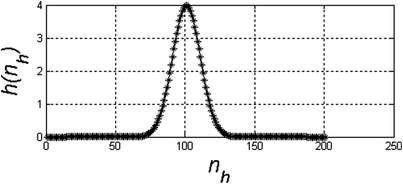
The results of the differentiation operation for m* = 50 calculated according to the formula (1.5) are shown in the table below (Table 1.1). As is apparent from the results shown in Table 1.1, calculating the derivative in the designated direction (in this case along the m-axis) in accordance with the definition does not produce the desired results. The image L(m, n) should be filtered out using any method, so that local changes in the pixel brightness will not affect the result. In this case, filtration is carried out through, for example, convolution of the image L(m, n) with the mask h(m _h, n _h), wherein the mask will be understood as the kernel, in this case, the Gauss transform, i.e.:

$h\left( {m_{h} ,n_{h} } \right) = \frac{1}{{2 \cdot \pi \cdot \sigma^{2} }}\exp \left( { - \frac{{m_{h}^{2} + n_{h}^{2} }}{{2 \cdot \sigma^{2} }}} \right)$

(1.7)

where σ is the standard deviation.

The filter mask has a resolution M _h × N _h = (2 · m _w + 1) × (2 · m _w + 1) with the centre of the coordinate system located at the point (m ₀, n ₀). On this basis, the convolution was carried out according to the known equation:

$L\left( {m,n} \right)*h\left( {m_{h} ,n_{h} } \right) = \sum\limits_{{m_{h} = m_{0} - m_{w} }}^{{m_{h} = m_{0} + m_{w} }} {\sum\limits_{{n_{h} = n_{0} - n_{w} }}^{{n_{h} = n_{0} + n_{w} }} {L\left( {m - m_{h} ,n - n_{h} } \right) \cdot h\left( {m_{h} ,n_{h} } \right)} }$

(1.8)

In the one-dimensional case, where m = const. (hereinafter referred to as m*), using the first derivative of the function and convolution operation enables to create the edge detector. Then the location of the edge can be determined after performing an elementary binarization operation on the waveform $\partial \left( {L\left( n \right)*h\left( {n_{h} } \right)} \right)/\partial n$ —Table 1.2.

Table 1.2

Various stages of edge detection using the gradient and convolution with the Gaussian kernel

Value	Image/Graph
L(m*, n)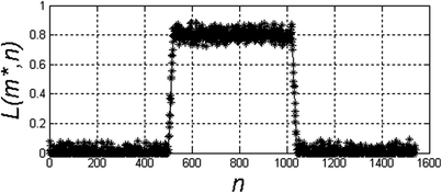
$h\left( {n_{h} } \right)$
L(n)*h(n _h)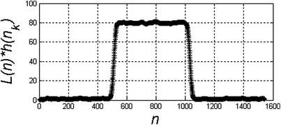
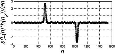$\frac{{\partial \left( {L\left( n \right)*h\left( {n_{h} } \right)} \right)}}{\partial n}$

On the basis of the problem formulated above (and Table 1.2), in practice, Roberts masks are defined directly from the differentiation definition (1.4), Prewitt masks—using the Taylor series expansion of the function L(m, n), and Sobel masks—taking into account the wheel proximity and Kirsch compass operator [40].

The second group of detectors is based on finding zero crossings of the second derivative of the function L(m, n). Similarly to (1.5) and (1.6), in the discrete case and with the shift on the n-axis, it can be written as:

$\frac{{\partial^{2} L\left( {m,n} \right)}}{{\partial n^{2} }}\,\hat{ = }\,\Delta _{n}\Delta _{n} = L\left( {m,n + 1} \right) - 2 \cdot L\left( {m,n} \right) + L\left( {m,n - 1} \right)$

(1.9)

similarly for the image axis m, i.e.:

$\frac{{\partial^{2} L\left( {m,n} \right)}}{{\partial m^{2} }}\,\hat{ = }\,\Delta _{m}\Delta _{m} = L\left( {m + 1,n} \right) - 2 \cdot L\left( {m,n} \right) + L\left( {m,n + 1} \right)$

(1.10)

As in the case of the first derivative, detectors based on the second derivative are very sensitive to the slightest change in grey levels. For this reason, pre-filtration with the Gauss filter is performed, yielding the results presented in Table 1.3.

Table 1.3

Various stages of edge detection using the second derivative and the Gauss filter