Besides the estimated STRFs (Fig. 37.1a), idealized STRFs modeled with 2D-Gabor functions are used to extract features that encode spectro-temporal modulations. In 2012, Schädler et al. proposed an approach in which a set of 2D-Gabor filters, suitable for ASR, is generated by means of a modulation filter bank (Fig. 37.1b). While the estimated STRFs show that the measured neurons are tuned to more ­complex patterns, the 2D-Gabor filters are simpler and only tuned to a specific ­combination of a spectral and a temporal modulation frequency. The spectro-­temporal features are extracted from the time-frequency representation by 2D convolution with the STRFs or 2D-Gabor filters. The filtered spectro-temporal representations contain the expected activation pattern of a neuron with the specific STRF at different center frequencies. The center frequencies are selected such that the STRFs or Gabor filters overlap, measured by the 2D correlation, and does not exceed a threshold. For STRFs, the threshold was set to 0.5; for the Gabor filter bank features, the values are taken from Schädler et al. (2012). The feature vector is composed of the output at the selected center frequencies. The dimensionality of the feature vectors for STRF and Gabor features is approx. 1,000 and 311, respectively.

To establish a valid comparison of human and machine performance, HSR and ASR results were obtained with the same speech database (noisy digit sequences from the Aurora2 corpus (Hirsch and Pearce 2000)). Results reported in this work were obtained by training the ASR system with a mixture of clean and noisy speech (“multi-condition training”). Testing is performed with clean and noisy digit strings using eight noises (four of which were used during training) with SNRs ranging from −5 to 20 dB. Speech items from 214 speakers were used for either training or testing. Ten subjects aged between 25 and 39 with normal hearing listened to the audio material in a sound-insulated booth via audiological headphones. Signals were presented at a comfortable listening level. Since Aurora2 test material contains more than 70,000 digit strings, a subset was compiled that is suitable for listening tests with humans. Pilot experiments were performed to identify the SNRs at which listeners actually produce errors. With clean signals, a 0 % error rate was obtained with a list containing 650 words, and even at 5 dB SNR, the error rate for two listeners was below 1 %. Hence, the tests with 10 listeners were performed at the lowest SNRs from the Aurora2 database (0 and −5 dB).

The Aurora2 reference ASR recognizer uses 13-dimensional MFCCs with delta and double-delta features, which are computed from the speech data using the front end provided with the hidden Markov toolkit. Results for PNCCs were obtained as a second baseline, since they are related to one of the time-frequency representations investigated in this work.

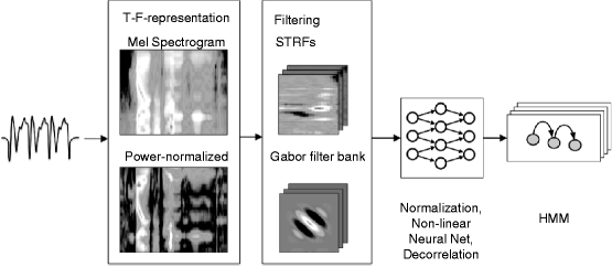
The resulting 39-dimensional features are used to train and test the hidden Markov model (HMM). Spectro-temporal features are used as input to a Tandem that consists of a nonlinear neural net (multilayer perceptron, MLP) and an HMM (Fig. 37.2). The MLP maps the input features to phone posteriors, which are decorrelated with a principal component analysis and fed to the HMM.

Recognition scores for humans, ASR baseline features, and ASR spectro-temporal features are presented in Table 37.1. The last column of Table 37.1 shows the speech reception threshold (the SNR at which 50 % of words are correctly identified). The SRTs were obtained by linear interpolation of recognition scores shown in Table 37.1 and Fig. 37.3.