(4.1)
for m ∈ (L K (n, i), L K (n, i) + p r9 ) and m i ∈ (1, p r9 ).
The image L GK (m i , n) is shown in Fig. 4.1.
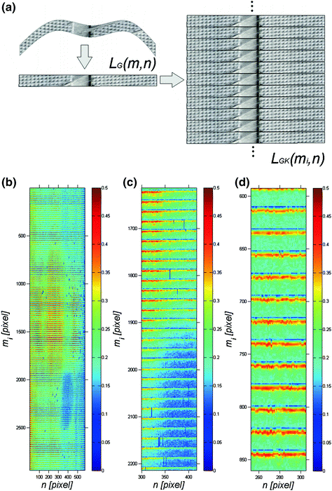

Fig. 4.1
Schematic diagram of rules of corneal texture conversion a actual image L GK (m i , n), b–d zoom of its selected fragments
Figure 4.1 shows the corneal texture separated from individual i images L G (m, n) for the adopted constant thickness p r9 = 20 pixels. Local shifts of recurrent elements of the corneal texture are visible in Fig. 4.1. Their further analysis involves the removal of the brightest and darkest rows using double-threshold binarization for which:


where:

(4.2)

(4.3)
L GKSM (m i ) the result of median filtering of L GKS (m i )
p r10 —threshold, adopted arbitrarily as 0.001, responsible for the tolerance range during double-threshold binarization, i.e.: L GKSM (m i ) + p r10 and L GKSM (m i ) − p r10.
The waveform of L BIN3 (m i ) has values equal to 0 for the extreme brightness of pixels calculated as the mean value for each row. A new image L GB (m k , n) is therefore a combination of the selected rows from the image L GK (m i , n). This selection was indicated by the value “1” in L BIN3 (m i ), i.e.:


(4.4)
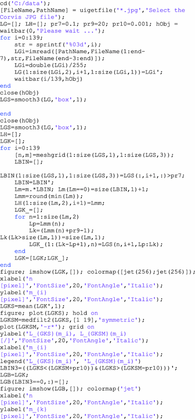
The source code allowing for the performance of the above calculations as well as the results are shown below (Fig. 4.2).
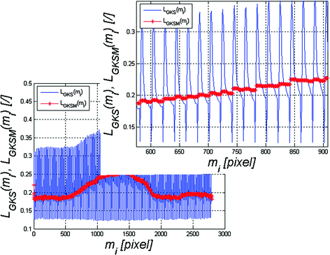

Fig. 4.2
Graph L GKS (m i )—blue, and graph L GKSM (m i )—red, with the zoom of a selected fragment
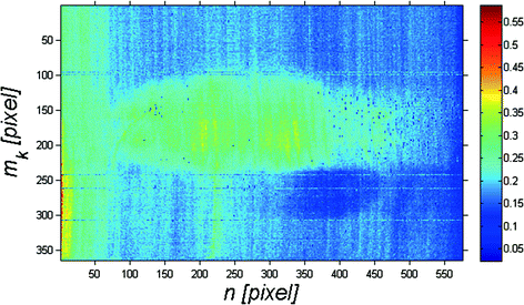
The graph L GKS (m i ) is the characteristic of the corneal texture both because of the contrast between the brightness values (minimum and maximum—Fig. 4.2) and the reproducibility obtainable for subsequent i images of the cornea. At this point, I encourage readers to trace the results obtained for L GKS (m i ) < L GKSM (m i ) and L GKS (m i ) > L GKSM (m i ). The removal of extreme brightness values in the described case provides the image L GB (m k , n) (Fig. 4.3) and enables to trace the brightness changes for successive values of m k . As shown in the illustrated image L GB (m k , n), there is a shift of typical texture fragments. The use of the Grey Level Co-occurrence Matrix (GLCM) provides information about local texture shifts during corneal deformation. The idea of using GLCM to evaluate statistical indicators of texture shifts is shown in Fig. 4.4.
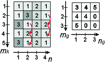

Fig. 4.4
Schematic diagram of calculating the matrix L GLCM (m g , n g ) (right) based on the sample matrix L GB (m k , n) (left) for p r11 = 1 in the vertical neighbourhood. Examples of counted vertical neighbourhoods of the values “1” and “2” are marked in red
The formal notation of the discussed method GLCM is shown below.

where:

for m k + p r11 ≤ M GB where M GB is the number of rows of the matrix L GB (m k , n).

(4.5)

(4.6)
The value p r11 is strictly dependent on the rate of changes in the texture content for subsequent i images. A preliminary analysis confirmed that the value p r11 should be absolute and lie in the range p r11 ∈ (M GB /40 M GB /10) pixels. The result, namely the image L GLCM (m g , n g ), for p r11 = M GB /40 is shown in Fig. 4.5.
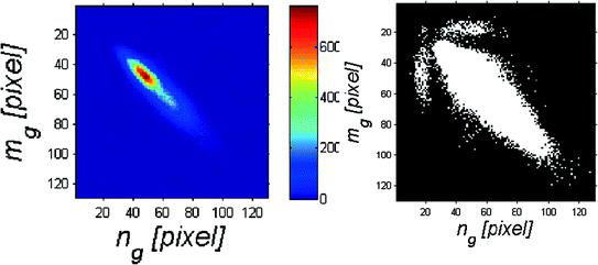

Fig. 4.5
Image L GLCM (m g , n g ) and its binary image being binarization with a threshold of 1 pixel
These images were obtained by continuing the subsequent phases of the algorithm operation with the notation:

Graycomatrix is a function that enables to obtain GLCM transformations. Parameters such as Offset allow for precise determination of the inclination angle at which the differences between pixels will be analysed—in this case p r11 = 10 pixels. Interpretation of the results is intuitive. The distribution of data on the main diagonal of the matrix L GLCM (m g , n g ) is directly related to the presence of vertical neighbourhoods between pixels of the same or similar brightness. The presence of data in the matrix L GLCM (m g , n g ) beyond the main diagonal is indicative of differences in brightness of vertically adjacent pixels. Thus, the shape of the distribution of data in the matrix L GLCM (m g , n g ) resembles an ellipse (especially after binarization—Fig. 4.5). Therefore, quantitative features directly related to changes in the corneal texture are the larger and smaller semi-major axes of the ellipse of the object from the image in Fig. 4.5b. Such measurement can be carried out using the function regionprop or imrotate in the following notation:

The results of the size of the larger and smaller semi-major axes are equal in the analysed case, d ED = 136, d ES = 75 pixels. The main parameter d ES is a quantitative measure of changes in pixel brightness for successive i images, for the area of the cornea. This is the first of the parameters defining quantitatively the eyeball response to an air puff and will be further referred to as w(1), i.e.: w(1) = d ES .
4.2 Analysis of the Eyeball Reaction
The outer contour of the cornea sequence L H (n, i) contains complete information on the response of the eye to an air puff. The contour is made up of three components:
constant component being the natural shape of the cornea—L HC (n, i),
eyeball reaction to an air puff—L HO (n, i),
corneal response to an air puff—L HR (n, i).
Analysis of the eyeball reaction is possible by analysing edges of the image L H (n, i). They correspond anthropometrically to the sclera fragments. However, the constant component, being the shape of the cornea and sclera fragments, is pre-separated for the initial images during acquisition.
The constant component is the natural shape of the cornea and is visible for the initial images in the sequence. Due to noise present in the image, it is good to average the shape of the cornea for several, several dozen of initial images L G (m, n, i). On the other hand, the start of the corneal deformation or the eyeball reaction is not precisely known.
The measure of differences is the adopted maximum of the standard deviation of the mean for the image L H (n, i), i.e.: L STDLH (i s ), measured as:


(4.7)
In subsequent iterations the value i s is increased starting from i s = 1. The algorithm stops its work when L STDLH (i s ) > 1 or if i s = 10, i.e.:
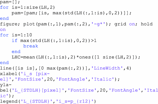
The obtained graph L STDLH (i s ) is shown in Fig. 4.6.
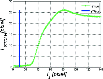

Fig. 4.6
Graph L STDLH (i s ) marked in green and threshold p r12 marked in blue
On the basis of the found i s , the waveform of the constant component L HC (n, i) was calculated, in simple terms independent of i (L HC (n)), in the following form:


(4.8)
The area i ∈ (1, i s ), from which L HC (n, i) was calculated from the waveform L H (n, i), is highlighted in red in Fig. 4.7.
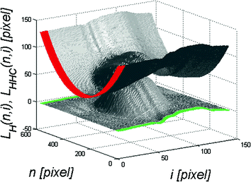

Fig. 4.7
Graph L H (n, i) (top) and L HHC (n, i) (bottom). The range i ∈ (1, i s ) is marked in red. The range from i = 1 to i s is marked in green
In the next step, using similar methodology, the eyeball reaction was calculated. For this purpose, in a preliminary stage, the waveform L HC (n, i) was subtracted from L H (n, i) thus obtaining L HHC (n, i), i.e.:


(4.9)
The waveform L HHC (n, i) is shown in Fig. 4.7 at the bottom. On its basis, the eyeball reaction will be calculated. As already mentioned, information from a sequence of images L G (m, n, i) on changes in the sclera position on both sides (the extreme columns) of the image will be used here. Since it was assumed that the sclera is not subject to deformation, changes in the position of the eyeball can be linearly reconstructed based on this information. Accordingly, the values of the standard deviation of the mean were calculated for the extreme positions of the columns, i.e., for example to the initial columns:


(4.10)
The first value n s , for which n s > 1, is the sought range n ∈ (1, n s ). On this basis, the linear reconstruction of changes in the eyeball position is performed—L HO (n, i), i.e.:


(4.11)
The characteristic areas of the edges L HHC (n, i) are shown in green in Fig. 4.7 at the bottom. An example of the resulting waveform L HO (n, i) is shown in Fig. 4.8 in blue.
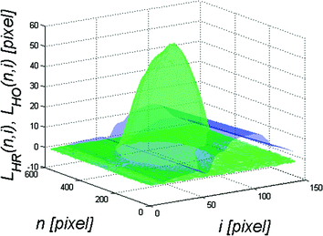

Fig. 4.8
Graph L HO (n, i) in blue and L HR (n, i) in green
The code of this fragment in Matlab is as follows:
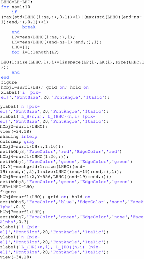
The new applied functions include linspace. The other functions have already been used before, such as: hold on intended to freeze the graph, grid on designed to show the rastr in the graph, surfl meant to show 3D graphs and their parameters FaceColor, EdgeColor etc.
On the basis of the waveform of the eyeball reaction L HO (n, i), it is possible to determine a number of useful features in data analysis, for example, for classification.
4.2.1 Distinction Between the Eye Position—Left/Right
Musculi bulbi oculi and the surrounding muscles respond differently to force in the form of an air puff. The eyeball is pushed into the skull. As a consequence, straight and oblique muscles withstand it. Mirror arrangement of these muscles for the left and right eye enables to automatically distinguish between them. This difference is written in the following way using L L/R :

where:


(4.12)

(4.13)

(4.14)
Figure 4.9 shows the graph L HOR (i) in red and L HOL (i) in green.
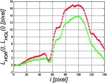

Fig. 4.9
Graph L HOR (i) in red and L HOL (i) in green
For the verified cases, when L L/R > 0, the left eye is analysed and in the other cases (L L/R < 0) it is the right eye. The situation when L L/R = 0 did not happen during the performed analyses. However, for L L/R ≈ 0, additional measurements and analyses should be conducted which would confirm whether the left or right eye was analysed. In extreme cases, such situations should be excluded from further analysis. The adequate notation is:

This feature, related to the ability to distinguish between the left and right eye, will also be mentioned in the next subchapter on the occasion of frequency analysis.
4.2.2 Frequency Analysis
Each of i images was acquired every 231 µs, which gives the acquisition frequency Fs = 4.33 kHz. Signal recording time is 231 µs * 140 images = 32.340 ms. The spectrum of the Fourier transform (FFT) L FFTHO is shown in Fig. 4.10 using the functions fft and nextpow2 (intended to designate the nearest power of 2 of the input vector length):
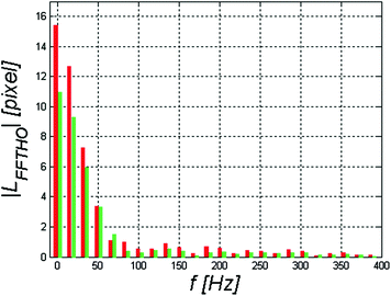

Fig. 4.10
Spectrum L FFTHO of the waveform L HOR (i) in red and L HOL (i) in green
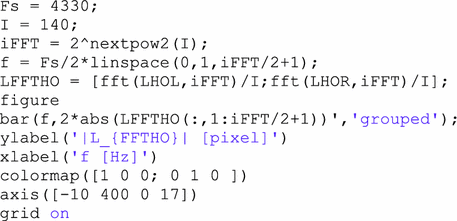
The results obtained are in line with expectations. There is no single dominant harmonic (Fig. 4.10). The spectrum of waveforms L HOR (i) and L HOL (i) may be divided into the range from 0 to 80, 90 Hz for the low frequency components and above 90 Hz for higher frequencies. However, a closer analysis of signals, for example using the Hamming or Blackman window, requires here the use of Matlab toolbox, namely Signal Processing, to which I refer interested readers.
Remaining in the area of the functions available in Image Processing toolbox, the convolution (function conv2) was further used to separate low-frequency components from higher frequencies of the waveform L HO (n, i). The convolution function (conv2) was used with the averaging filter mask h 5 having a resolution M h5 × N h5 = 19 × 19 pixels. The mask size, due to the large separation of low frequencies from the high ones (Fig. 4.10), may vary considerably even to M h5 × N h5 = 29 × 29 pixels, which does not significantly affect the results obtained. The source code fragment responsible for the division of L HO (n, i) into L HOH (n, i) containing high frequencies and L HOW (n, i) containing low frequencies is presented below:

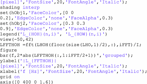
The results obtained are presented in Figs. 4.11 and 4.12.
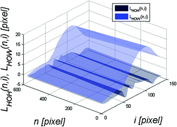
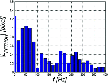

Fig. 4.11
Graph L HOH (n, i) in black and L HOW (n, i) in blue

Fig. 4.12
Spectrum L FFTHOH of the waveform L HOH (i)
From a practical point of view (medical practice), scalar values which describe the maximum amplitude of the low and high harmonics as well as the waveforms L HOH (i) and L HOW (i) are vital. These values are further parameters which quantify the eyeball response to force in the form of an air puff, i.e.:


(4.15)

(4.16)

(4.17)
These features will be used further for a comprehensive, quantitative assessment of the eyeball reaction to an air puff from the Corvis tonometer.
4.3 Analysis of the Corneal Response
The corneal response L HR (n, i) is designated based on the information acquired in the previous subchapter, i.e.:
 < div class='tao-gold-member'>


Only gold members can continue reading. Log In or Register to continue
Stay updated, free articles. Join our Telegram channel

Full access? Get Clinical Tree


