(57.1)
where x i , i = 1, …, N, are observed neural activities; K is the number of sources; θ k , k = 1,…, K, are parameters (mean and variance) of component Gaussian distributions; and π k , k = 1, …, K, are the mixture weights. The computational goal of ASA in this framework is to estimate the parameters of the GMM, θ and π, which best match the distribution of neural activities corresponding to each source. In the case of streaming in particular, the goal is simply to judge the number of sources from the observed neural activities. For example, in the classic ABA tone sequence, two hypotheses may be generated: both A and B coming from a single source (one stream) or A and B coming from different sources (two streams).
The system judges which hypothesis is more plausible based on the observations. The GMM parameters, θ and π, are estimated using the Bayesian inference. Posterior probability (“belief”) about perceptual state (Z, π, θ) after the data X are observed is computed by

where Z is a set of hypotheses, P(θ)P(π) is the prior belief about sources (i.e., the Gaussian mixture parameters and weights), and P(X | Z, θ)P(Z |π) is the likelihood. Using this Bayesian updating, the GMM parameters are renewed each time a new data point X is observed.

(57.2)
We applied this model to the ABA sequence with various combinations of frequency separation (Δf) and tone SOA (ΔT) (Fig. 57.1). Note that the actual value of Δf is not critical here, and Δf could be replaced with any feature that is represented on a continuum. The memory span of the system was set to 200 (arbitrary unit, common to ΔT; if ΔT is 10, data for 20 tones (=200/10) are stored in the system). Of special interest here is the effect of W, one of the parameters of P(θ). In theory, the smaller the value of W, the stronger is the tendency for the system to model the observed data with a small number of Gaussian distributions with large variances. This prediction was confirmed by the simulation results; with W = 0.1 (Fig. 57.1a), the integration-segregation boundary was similar to the behavioral coherence boundary in van Noorden (1975), and with W = 10, it was similar to the behavioral fission boundary. Thus, the parameter W may be considered as corresponding to the response set or volitional control of the listener. We introduced random fluctuations in W (W = 10w, where w is derived by applying a low-pass filter to a Gaussian noise with a mean of 0 and a standard deviation of 1). The fluctuation of W is not totally unrealistic, because neural activities are stochastic and sensory observation is not always clean. With an appropriate parameter setting, the fluctuated W qualitatively simulated the “ambiguous zone” in van Noorden (1975) (Fig. 57.1d).
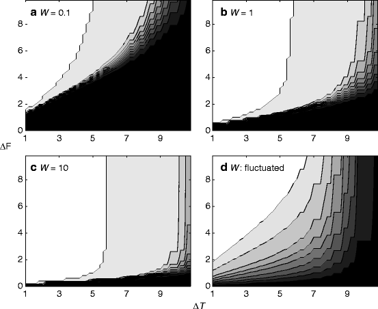

Fig. 57.1
Probability of “segregation” judgment (coded as brightness) as a function of tone SOA (∆T) and frequency separation (∆F), calculated with three values (0.1 (a ), 1 (b ), and 10 (c )) of W and fluctuated W (d). The units of ∆F and ∆T are arbitrary
In this model, the statistical power increases with the number of observed data, leading to the “segregation” judgment. Figure 57.2 shows the probability of “segregation” judgment as a function of the number of observed tones (equivalent to time). Without the fluctuation of W, the change of Δf resulted in simple horizontal shifts of the same curve (Fig. 57.2, left), which is inconsistent with the behaviorally observed buildup of streaming. With the fluctuated W, on the other hand, the simulated curves resembled the behavioral ones, in terms of the dependence of the curve shape on Δf (Fig. 57.2, right).
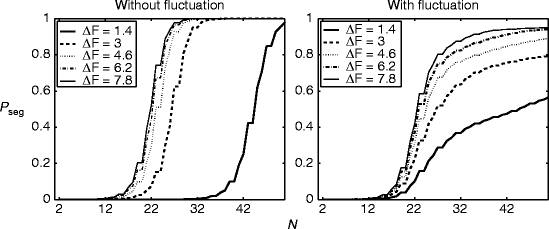

Fig. 57.2
Simulated buildup of streaming with (left) and without (right) the fluctuation of W. Probability of “segregation” judgment is plotted as a function of the number of observed tones N (equivalent to time). The unit of ∆F is arbitrary
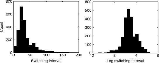
The fluctuation of W also results in multistable perception. The same combination of Δf and ΔT can yield different perceptual states due to the transient boundary shift caused by the fluctuation of W. Figure 57.3 shows the histogram of switching intervals simulated by the model with the fluctuated W. The log-normal distribution was the best fit among several probability distributions including the gamma and normal distributions. This is consistent with behavioral data (Kashino et al. 2007).
