Biostatistics
Simon Hollands MD, MSc (Epid)
Sanjay Sharma MD, MS (Epid), FRCSC, MBA
Hussein Hollands MD, FRCSC, MSc (Epid)
Introduction
In Chapter 1 various study designs were discussed in order to provide an overview of some of the more common methodologic approaches used in evidence-based medicine for determining the efficacy and effectiveness of drugs, treatments, and procedures in ophthalmology. In order to objectively examine the literature it is important to gain an understanding of the statistics that will be reported so that informed interpretations that are both unbiased and clinically relevant can be made.
In this chapter we explain the principles of hypothesis testing and statistical significance and discuss some of the more common statistical approaches used to report findings in the ophthalmology literature.
Hypothesis Testing, Statistical Significance, and Clinical Significance
Traditional statistical inference is based on hypothesis testing. To understand the framework that underlies this process, it is constructive to consider the sample of study patients in the context of the larger, true population of interest. Since it is not feasible to obtain data on an entire population, the next best alternative is to make inference about the population of interest based on statistics from a (random) sample of individuals that are representative of the target population.
Initially a null hypothesis is made (denoted by H0); statistical tests are then carried out on the study sample to provide evidence in favor of rejecting or accepting H0. The null hypothesis states that there is no difference between groups with respect to the outcome of interest, or that a given factor does not affect the outcome. For example smoking is harmless, or monthly ranibizumab has no effect on visual acuity for patients with neovascular age-related macular degeneration (AMD). In the case of a randomized controlled trial (RCT), H0 assumes that the intervention has no effect, or that the outcome is the same in all treatment arms. The Minimally Classic/Occult Trial of the Anti-VEGF Antibody Ranibizumab in the Treatment of Neovascular Age-Related Macular Degeneration (MARINA)1 was a landmark RCT that investigated the effect of monthly intravitreal injections of ranibizumab (0.3 mg and 0.5 mg) versus control (sham injections) for the treatment of exudative AMD. In the MARINA trial, the null hypothesis was that on average sham injections produced the same change in visual acuity over 24 months as did monthly injections of ranibizumab.
Statistical tests provide a measure of how likely it is for the observed study results to have occurred under the assumption that the null hypothesis was true (i.e., no true effect existed). In other words, hypothesis testing measures the probability that the results occurred simply by chance. If the probability is low enough, then H0 is said to be rejected in favor of the alternative hypothesis: Ha that the factor being examined does in fact have an influence on the outcome of interest.
Statistical Significance
In evidence-based medicine results are generally considered statistically significant at the 5% level. As a probability, the significance level is referred to in the literature as α, which
is the probability of committing a type I error. A type I error occurs if the null hypothesis is rejected when it is actually true (i.e., no true treatment effect exists, yet the statistical test concluded the result was statistically significant). It can also be thought of as a false positive. At α = 0.05, by chance alone, if a trial were repeated 100 times then findings with an effect as great, or greater would be found 5 times (under the assumption of H0). In the literature, the level of statistical significance is generally reported either by a p-value, or a 95% confidence interval (CI). The 95% CI corresponds to (1— α), which is the probability of correctly rejecting a null hypothesis.
is the probability of committing a type I error. A type I error occurs if the null hypothesis is rejected when it is actually true (i.e., no true treatment effect exists, yet the statistical test concluded the result was statistically significant). It can also be thought of as a false positive. At α = 0.05, by chance alone, if a trial were repeated 100 times then findings with an effect as great, or greater would be found 5 times (under the assumption of H0). In the literature, the level of statistical significance is generally reported either by a p-value, or a 95% confidence interval (CI). The 95% CI corresponds to (1— α), which is the probability of correctly rejecting a null hypothesis.
A p-value is useful in that it provides the actual probability that the events occurred by chance (i.e., probability of rejecting a true H0). For example, in the MARINA trial1 a p-value of < 0.001 was reported comparing visual acuity outcomes between the ranibizumab and the sham-injection groups after 12 months. Specifically, one of the main findings was that 94.6% of the patients receiving 0.5 mg ranibizumab lost fewer than 15 letters from baseline as compared with 62.2% in the sham-injection group; this corresponds to an absolute risk reduction (ARR) of 32.4% (treatment proportion [94.6%] – control proportion [62.2%]). The p-value of < 0.001 is calculated from a statistical test on the difference in these proportions (or ARR). Thus, the probability that a difference of 32.4% (treatment proportion – control proportion) or greater would be found by chance alone—if H0 was true—is less than 1 in 1,000 (i.e., p < 0.001) implying strong evidence for a treatment effect. A null hypothesis can never be proven true or false since an entire population is never analyzed; a p-value measures the strength of evidence against the null hypothesis.
A 95% CI is often more clinically relevant than a p-value, as it defines an actual interval for which the true value is likely to lie. The smaller the CI the more precise the estimate. A CI and a p-value convey similar information. For instance a 95% CI for a difference in proportions (means) that does not contain 0 would be statistically significant at the 5% level (i.e., p ≤ 0.05). A 90% CI would parallel a p-value ≤ 0.1. If the sample size is known then a CI can be derived from a p-value and vice versa (given that the statistical test used is also known).
It is also important to understand the relationship between sample size and statistical significance. This relationship is related to the probability of committing a type II error. A type II error occurs when the statistical test fails to reject a null hypothesis that is actually false. It can be thought of as a false negative whereby a true difference between treatment groups exists but the difference is not found to be statistically significant. To conceptualize type I and type II errors it is useful to consider the following table:
|
The probability of a type II error occurring is denoted by β and is highly related to the power of a statistical test (1 — β). The power (generally 80%) refers to the likelihood of not committing a type II error. The sample size plays a key role in determining this probability. As the sample size is increased, it becomes less likely that a true difference between groups will not be shown to be statistically significant.
It is important to realize that the conventional cut-point of α = 0.05 that denotes statistical significance is actually an arbitrary value. If this cut-off is used absolutely then a p-value of 0.051 would be classified as not statistically significant whereas p = 0.049 would be statistically significant. Low p-values and narrow CIs are a direct function of larger sample sizes. Therefore in a small study, an effect that may in fact be clinically relevant may not be statistically significant. The converse can also occur; with a large enough sample size any true treatment effect, no matter how small, can be shown to be statistically significant. Therefore, in addition to the
statistical significance of a treatment effect it is important to look at the clinical (or practical) significance of that effect.
statistical significance of a treatment effect it is important to look at the clinical (or practical) significance of that effect.
Clinical Significance
The clinical (or practical) significance of a result refers to the level of effectiveness of a treatment at which a clinician feels adoption of the treatment would be justified in clinical practice. For instance, an ophthalmologist may feel that to justify the cost and risk of adverse events for a particular treatment it should confer a relative risk (RR) of 0.5 or less for a loss of 15 or more letters of distance visual acuity. In this case, if an RR of 0.5 or less was shown in an RCT to be statistically significant (i.e., p <= 0.05) then the intervention should be considered for use. However, a larger sample size (and thereby more outcome events) in an RCT leads to more confidence in the results and hence more precision. Practically, this means a smaller p value or a narrower 95% CI. In fact, any treatment effect, in theory, can be found to be statistically significant through an RCT if enough people are studied. Therefore, when interpreting a result, the clinician should decide on an RR (or treatment effect) that is practically significant for the clinical application of the study. Then, if the results show a statistically significant treatment effect equal to or greater than the practically significant cutoff point, the clinical intervention may be considered for use. As discussed in the section on sample size calculations, if a given treatment effect is practically but not statistically significant, then the study is inadequately powered and no useful conclusion can be made. Conversely, if a treatment effect is statistically significant (for example in a large study) but not clinically significant then the intervention would not be implemented even though it had true effectiveness since the magnitude of the effectiveness was inadequate.
The next two sections explore some of the more common measures for reporting efficacy, highlighting the different approaches for when dichotomous and continuous outcomes are considered.
Dichotomous Outcomes
By definition, a variable that has two categories (e.g., male/female) is dichotomous. In ophthalmology some outcomes are inherently dichotomous such as adverse events following certain treatments (e.g., occurrence of endophthalmitis after ranibizumab). For measuring efficacy, however, it is more common for variables to be categorized based on meaningful cutoff points of continuous variables. For instance many clinical trials will define an event such as a 15-letter loss of visual acuity as a harmful occurrence of interest. The study is then designed to test the (null) hypothesis that the proportion of individuals with a 15-letter loss in visual acuity is the same between intervention groups.
For dichotomous outcomes, the frequency of clinical outcomes between groups is of primary interest and the effect can be measured based on the risk or the odds of an event occurring. Generally, the measure of effect is reported in either relative terms (i.e., RR or odds ratios [OR]), or absolute terms (through risk differences). The terms “risk” and “odds” are often used interchangeably in the literature; however, the term “risk” implies an actual probability of the outcome occurring, and can only be calculated in certain instances. Specifically if a study captures the temporal sequence (or cause and effect) of the exposure and outcome, as is the case in most RCTs and cohort studies, then results can be reported in terms of risk.
Measures of Risk
The size of the treatment effect versus a control group can be reported as an RR. A risk ratio is another common term for this measure with the same abbreviation (RR). RR is straightforward to calculate, as it is simply the incidence rate (risk) in the treatment (experimental) group divided by the incidence rate (risk) in the control group. It can be thought of as the ratio of the probability of the event occurring in the treatment group compared to the control group. It takes on any value greater than zero.
An RR = 1 (unity) means that there is no difference in the probability of an event occurring between the exposed (treatments) and unexposed (control) study groups. A 95% CI is generally reported alongside the RR to provide a measure of precision (or statistical
significance). If the 95% CI does not cross 1, then the H0: RR=1 is said to be rejected, and the RR is statistically significant at the 5% level (i.e., p< 0.05).
significance). If the 95% CI does not cross 1, then the H0: RR=1 is said to be rejected, and the RR is statistically significant at the 5% level (i.e., p< 0.05).
Given a defined outcome and a defined exposure (or treatment), an RR > 1 means that the probability (risk) of the outcome occurring is greater in the exposed (treatment) group versus the unexposed (control) group. Conversely, an RR < 1 suggests that the risk of the outcome occurring in individuals that are exposed (treated) is lower than those who are unexposed (control). The further from unity (in either direction) the greater the magnitude of the treatment effect. When interpreting an RR for direction of the treatment effect one must distinguish whether the outcome of interest is beneficial (e.g., losing 15 or fewer Early Treatment Diabetic Retinopathy Study [ETDRS] letters of distance visual acuity) or harmful (e.g., endophthalmitis). Another related measure, which in some cases has a more intuitive interpretation, is the relative risk reduction (RRR). When an RR is less than unity, it means that an exposure (treatment) has a protective effect against the outcome; the RRR is used to report the size of the risk reduction. The RRR is calculated as (1-RR), and generally expressed as a percentage. For example, if a treatment confers an RR of 0.9 for a particular outcome, the RRR would be 0.1 or 10% (i.e., 1-0.9).
Results are often conveyed with complex figures and statistical analyses; however, it is often easiest to convert the main study results into a simple 2×2 contingency table as demonstrated in Table 2.1 to allow for clearer conceptualization. From the contingency table, several measures of effect can be calculated. As an example, we consider the results of the MARINA1 trial where the intervention is monthly intravitreal injections of 0.5 mg ranibizumab and the control is sham injections. One dichotomous outcome of interest was whether or not patients lost > 15 ETDRS letters over 12 months’ follow-up. The RR and RRR comparing the risk of losing > 15 ETDRS letters between treatment arms were not explicitly reported in the study. However, a contingency table can be derived from the data given in the manuscript (Table 2.2)<SPAN title="2 × 2 table was derived from Figure 2.1 by working backwards from the information given: Total sample receiving the sham (n = 238) and 0.5 mg ranibizumab (n = 240) injections, and the percentage of patients who lost * and the effect measures of interest can be calculated by the reader using the formulas provided at the end of the chapter (Table 2.3). The RR and RRR are calculated as follows:
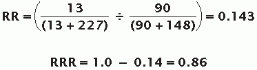
The RR of 0.143 indicates that patients receiving ranibizumab had a lower probability of losing more than 15 ETRDS letters (a “harmful outcome”) than patients who were given the sham injections. The ranibizumab injections lowered the risk of the harmful outcome occurring by 86% (RRR = 1.0 – 0.14 = 0.86).
TABLE 2.1 Standard 2×2 Contingency Table | ||||||||||||
|---|---|---|---|---|---|---|---|---|---|---|---|---|
|
Stay updated, free articles. Join our Telegram channel

Full access? Get Clinical Tree


