Arterial Input Function and Venous Output Function
Soren Christensen
Matus Straka
Ting-Yim Lee
Introduction
The Role of the Arterial Input Function and Venous Output Function in Perfusion Measurements
The arterial input function (AIF) is the concentration-time curve of the contrast agent (indicator) measured in an arterial vessel that feeds the organ of interest. Similarly, the venous output function (VOF) is the indicator concentration-time curve measured in a vein that drains the organ of interest (Fig. 26.1). These functions are key components of the convolution model (see Chapter 24), which is the prevailing model of how tissue concentration-time curves can be used to infer perfusion parameters. The AIF is essential for absolute quantification of hemodynamic parameters, such as cerebral blood flow (CBF), cerebral blood volume (CBV), and mean transit time (MTT). Because arteries from which AIFs are selected are usually of smaller caliber, a VOF is often used to correct the AIF for partial volume artifacts.
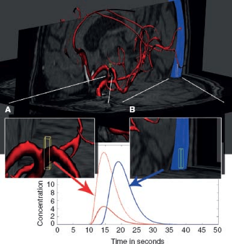 FIGURE 26.1. Arterial (red) and venous (blue) cerebral vessels with two voxels (yellow cubes) positioned over an artery and a vein. Inset A shows a voxel of approximately 2 × 2 × 5 mm that does not completely encompass the middle cerebral artery (MCA). Inset B shows a voxel completely enclosed in the sagittal sinus. Plot: The red stippled line shows the actual concentration-time curve of tracer agent inside the artery. The solid red line shows the concentration-time curve measured from the entire voxel, which is smaller than the actual concentration because the voxel only partially covers the vessel. However, the concentration-time curve measured in the voxel has the correct shape (if we neglect signal from tissue outside the vessel) and differs from the real AIF by only a scale factor proportional to the fraction of the voxel taken up by the vessel. The venous voxel is fully contained in the vein and therefore reflects the true concentration in the vein. The bolus fractionation principle states that the area under the bolus curve is equal anywhere inside all vessels in the system, so the true arterial input function (AIF) and venous output function (VOF) have identical areas under the curve. Therefore, the VOF area can be used to rescale the AIF to its true magnitude. |
The AIF can be thought of as a “supply” function that describes the delivery of the tracer agent over time into the tissue that is being imaged. Each imaged voxel of tissue retains the contrast agent for a variable period as it crosses the vascular bed, and this retention is seen as a smearing or dispersion of the AIF concentration-time curve. In other words, the tissue concentration-time curve in each voxel is a dispersed form of the AIF. The goal of deconvolution is to characterize the exact nature of this dispersion, as this will reveal the MTT through the tissue of each voxel and also allow for calculation of CBV and CBF. More formally, the nature of the dispersion that takes place in each voxel is determined by the characteristic retention profile of the tissue, or the impulse residue function. Once the impulse residue function is known, the CBF, CBV, and MTT can be estimated (see Chapter 24).
With image resolution of today’s magnetic resonance imaging (MRI) and computed tomography (CT) systems, it is often not possible to find a voxel that is fully contained within an artery, and this means that a measured AIF is subject to some degree of partial volume effect from adjacent tissue. In other words, the blood volume in the arterial voxel is not 100%. This in turn leads to underestimates of the tracer concentrations and ultimately to overestimates of CBF and CBV (Fig. 26.1). The VOF can be used to correct the AIF by a simple rescaling procedure. The so-called “bolus fractionation principle” states that the area under the first-pass concentration-time curve is identical in all vessels downstream to the bolus inlet site.1 Therefore, the areas under the concentration-time curves of the AIF and VOF are expected to be identical as long as the tracer remains intravascular:
Partial voluming causes a downscaling of the AIF concentration that is proportional to the fraction of the voxel occupied by the arterial vessel.
A comparison of the area under the AIF and VOF will reveal the extent of AIF concentration underestimation
and—when one assumes the area under the venous and arterial time course should be the same—the correction is a simple rescaling to bring the AIF up to the same area under the concentration-time curve as the VOF:
and—when one assumes the area under the venous and arterial time course should be the same—the correction is a simple rescaling to bring the AIF up to the same area under the concentration-time curve as the VOF:

The area under the VOF is subject to less partial volume effect due to the larger caliber of venous vessels.
This correction scheme assumes that partial volume artifacts give rise to a simple downscaling of the AIF, which is a reasonable assumption for CT perfusion, but for dynamic susceptibility-contrast (DSC)-MRI the situation is more complex, as is discussed later in this chapter.
The AIF selection can have a significant effect on the calculated perfusion values; this chapter reviews the physical and physiologic phenomena that challenge a correct determination of the AIF as well as proposed correction schemes. Sections 2, 3, and 4 cover concepts that are in large part general to both CT and MR acquisitions, whereas Sections 5 and 6 deal with AIF issues that are specific to each modality.
This chapter focuses on CT contrast perfusion and MRI dynamic susceptibility perfusion of the brain, but most of the concepts have relevance for perfusion of other organs.
Historical Background and Chapter Outline
Measurements on indicator agents in biological systems date back to G. N. Stewart’s experiments on cardiac output in 1897, in which electrical resistance was used to measure the concentration of an injected saline infusion.2 Indicator methods have since been used extensively in circulation physiology research, diagnosis, and monitoring. Early experiments were limited to whole-organ flow measurements by direct sampling of blood to determine indicator concentrations. However, current imaging techniques—single photon emission computed tomography (SPECT), CT, and MRI—allow for measurement of indicator concentrations noninvasively and spatially resolved to the resolution supported by the imaging hardware.
The theoretical basis for CT perfusion processing with image-based AIF measurements was described and employed by Leon Axel in the early 1980s.3,4 Hardware developments over the following decades provided better coverage and higher resolution imaging and brought CT perfusion imaging into general clinical use with on-console software to measure the AIF and VOFs required for quantification.
In the late 1980s, dynamic susceptibility contrast agents and fast imaging techniques put MR-based perfusion measurements at an advantageous position compared to CT imaging, in terms of both image coverage and signal-to-noise ratios (SNRs) of the contrast agent measurements. This paved the way for perfusion sequences with more coverage and better SNRs than what was offered by CT perfusion at the time.5 For this reason the majority of methodologic and clinical research in bolus-tracking imaging has taken place using MRI perfusion imaging, but with newer, multidetector CT systems capable of whole-brain perfusion imaging, the gap between the two modalities is narrowing.
In the mid-1990s, several methods to obtain CBF and MTT estimates by deconvolution with an AIF were proposed, and the AIF deconvolution method became the preferred way of measuring perfusion.6,7
Many clinical studies have since employed deconvolution methods using an AIF that was manually selected based on the appearance of the concentration-time curves, usually averaged from 1 to 10 pixels with the appropriate signal characteristics.
It later became clear that the site of AIF selection had a significant effect on the perfusion estimates, and this prompted several groups to propose automated means of identifying the AIF to provide more reproducible maps; this is reviewed in Sections 2 and 3 of this chapter.8
It also became clear that use of a single AIF for the whole organ, often termed a global AIF, can introduce considerable error into the perfusion maps, particularly in patients with acute stoke and patients with steno-occlusive disease.9 Even if the measured AIF is a good estimate of the arterial concentration-time curve in the vicinity of its measurement, it may not be a good representation of what the AIF looks like further downstream, closer to the tissue where the AIF can be both delayed and dispersed (see Local AIF Techniques). In principle, the most straightforward solution to the problem of an unrepresentative, global AIF is to select multiple AIFs locally, close to the tissue, and to deconvolve each voxel with the AIF estimated to feed it. Such techniques are known as local AIF techniques and are covered in section 4. However, often the arterial feeder for a given tissue voxel is not fully known due to anatomic variants or pathology. In an acute setting, the local supply routes can also change dramatically, such as seen with collateral flow.
Finding an AIF
AIF and VOF features
For an AIF to provide an accurate estimation of perfusion in a voxel, it must be an accurate reflection of the actual AIF that enters the voxel. In practice, the AIF is determined by one measurement, or as the average of several measurements of concentration-time curves in the proximal cerebral arteries, with the inherent assumption that a single AIF is representative of the AIFs feeding each voxel. This assumption is often incorrect and leads to errors in calculation of CBF and MTT as is discussed in
section 3. Despite these known issues with the method, use of a single, global AIF selected from the proximal vasculature remains the most prevalent technique in use today in commercial software as well as in published studies. The main reasons for the continued use of a single global AIF are likely founded in the complexity and lacking validation of newer, automated methods for multiple local AIF detection. In addition, maps created using a global AIF are more sensitive to hemodynamic disturbances in general, which are sometimes useful clinically, and absolute blood flow quantitation is secondary. Sections 4 and 5 on delay and dispersion and local AIF discuss how perfusion maps are affected by removal of delay and dispersion.
section 3. Despite these known issues with the method, use of a single, global AIF selected from the proximal vasculature remains the most prevalent technique in use today in commercial software as well as in published studies. The main reasons for the continued use of a single global AIF are likely founded in the complexity and lacking validation of newer, automated methods for multiple local AIF detection. In addition, maps created using a global AIF are more sensitive to hemodynamic disturbances in general, which are sometimes useful clinically, and absolute blood flow quantitation is secondary. Sections 4 and 5 on delay and dispersion and local AIF discuss how perfusion maps are affected by removal of delay and dispersion.
In the absence of signal-distorting artifacts, arterial and venous concentration-time curves can be identified anatomically, and based on their shape and area under the concentration-time curve from tracer kinetic principles: (a) Voxels covering arteries and veins have larger areas under the concentration-time curve than tissue voxels. This follows directly from the tracer kinetic theory, which states that the area under the concentration-time curve is proportional to CBV. (b) Arterial voxels will be the first to receive tracer agent and show nonzero concentration-time curves, that is, the delay to tracer arrival is short. After the arterial arrival, the tracer enters the tissue and then finally gets drained from the tissue by the veins. Another useful property is the first moment (temporal mean) of the concentration-time curve. The first moment will be lowest in the arteries, higher in tissue, and even higher in the veins. From statistics we know that the first moment of a probability distribution function—in our case the AIF and VOF can be seen probability distribution functions for the contrast agent passage times—yields the population mean transit time of the tracer transit. In other words, an AIF has a relatively large area, early arrival, and a narrow curve shape. A venous curve will also have high area, and in general a larger area under the curve than the AIF curve due to less partial voluming. The venous curve will be delayed relative to the AIF and often appears broader than the AIF, the latter owing to dispersion during the passage through the tissue. Figure 26.2 illustrates how these enhancement curve properties are determined.
Both the AIF and VOF have a prominent peak from the first-pass bolus passage, followed by a recirculation peak of less than half the magnitude of the first peak. Deviations from this pattern, for instance a dual-peaked appearance of the first-pass bolus or concentrations below 0, are often indicative of artifacts, such as patient motion, off-resonance induced pixel shifts, and T1 shortening. A number of artifacts can affect the AIF and VOF readings, many of which are specific to the imaging modality. Particularly DSC-MRI is subject to complex signal distortions that can change the shape of the AIF and VOF in a way that cannot be immediately identified as artifactual, and some of the aforementioned criteria can result in the selection of distorted AIF curves as discussed in the section on DSC-MRI artifacts.
Manual AIF and VOF Selection
The practice of manual AIF selection is based on practical and theoretical considerations.
 FIGURE 26.2. Concentration-time curves can be summarized by a number of features that will help decide whether the curve is of arterial, venous, or tissue origin. Common parameters are arrival time, time to peak (TTP), first moment, full-width-at-half-maximum (FWHM), and the area under the curve. These parameters can be determined either directly from the concentration data points (red curve), or from a fit to a gamma-variate function (black curve), which will normally produce more accurate results. The gamma variate fit is often adjusted to not cover the recirculation phase, which improves the accuracy of the estimated parameters. |
A global AIF is usually selected from a given anatomic region, for example, the M1 or M2 branches of the middle cerebral artery (MCA) in MR studies, or from the anterior cerebral artery in CT studies where coverage on most current systems are limited.8,10 In clinical studies of stroke, the AIF is often selected in the hemisphere contralateral to the abnormality, which provides the most
sensitive reference area to capture any hemodynamic abnormality, but this is inherently susceptible to potential bias from not capturing the delay and dispersion ipsilaterally. The manual AIF selection process varies widely with the software used, but it often involves an interactive interface where the user is able to explore concentration-time curves in an anatomic region visually and then select curves that exhibit the arterial characteristics listed previously.
sensitive reference area to capture any hemodynamic abnormality, but this is inherently susceptible to potential bias from not capturing the delay and dispersion ipsilaterally. The manual AIF selection process varies widely with the software used, but it often involves an interactive interface where the user is able to explore concentration-time curves in an anatomic region visually and then select curves that exhibit the arterial characteristics listed previously.
The VOF can be selected in an analogous fashion, guided by the outlined curve shape properties. Here, the VOF is often chosen from the sagittal or transverse sinus, focusing on the curve with the highest area.
Automatic AIF Detection Algorithms
In principle, automatic selection of a single, global AIF offers several advantages over manual AIF selection. Manual AIF selection requires availability of a trained operator to process the maps, but even with trained operators and the aforementioned criteria for shape and timing of concentration curves in place, it is highly unlikely that independent operators select identical AIFs and consequently produce the same perfusion maps. This lack of reproducibility is obviously not desirable. Automatic AIF selection addresses these issues and allows for quick and reproducible perfusion maps without the need for specially trained operators. A number of automated detection algorithms have been proposed over the years, but no single method has gained traction as a standard tool for scientific or clinical purposes. Most of the AIF detection algorithms that have been suggested to date are deterministic and will produce identical perfusion maps every time they are run on a given data set. A few algorithms rely on random starting points for the AIF detection algorithms, and these may not always produce completely identical maps when processing is repeated. It is important to note that reproducibility does not imply accuracy and that reproducibility by itself is of limited merit when assessing the efficacy of an automated method.
The major features of AIF-detection algorithms can broadly be divided into two stages: (a) Summary curve parameter extraction and (b) AIF candidate selection.
In the parameter extraction process, the concentration-time curves of each voxel are summarized by properties of the bolus shape, such as time-to-peak, bolus width, and arrival time. The AIF candidate selection process then identifies a limited subset of voxels with bolus shapes within a certain range consistent with AIF signal characteristics, such as early arrival, high peak, and narrow width. The cut-offs for what represents a value consistent with an AIF is often defined relative to the distribution in all voxels rather than by the absolute values of the features, since these can vary widely with the experimental conditions. For instance, width of the bolus, time to peak, and bolus height are clearly related to injection protocol and a number of other extracerebral factors, so absolute thresholds cannot be predefined.
Often the bolus properties are determined by fits to a gamma-variate function, but other types of functions have also been used.11,12 In techniques based on cluster analysis, the features considered are the very concentration-time curves that are divided into a low number of groups (clusters), where voxels with similar concentration-time curves are grouped together. The average concentration-time curve of each cluster is then summarized by measures of bolus shape; this is then used to select the cluster with the properties most consistent with arteries.13,14 Most automatic techniques presented in the literature have been assessed by how well they correspond to maps generated by manual AIF detection, implicitly using a manual AIF selection as a gold standard.11,12,13,14,15
In principle, AIF detection techniques can be assessed by comparing the produced perfusion maps to a gold standard reference perfusion image to see if a given AIF detection strategy improves correspondence with the gold standard perfusion map. A gold standard reference could in principle be obtained by other perfusion imaging modalities, such as positron emission tomography (PET), xenon-enhanced CT, and arterial spin labeling, but so far this approach has been limited owing to the difficulty in obtaining these images in quick succession.
It has been demonstrated that artifacts arising from the complex nature of the DSC-MRI signal formation can give rise to artifactual curves that are sharper than the actual concentration-time curve, and therefore lead to erroneous selection of AIFs if one is to purely select an AIF based on shape characteristics. Additional steps are needed to detect such artifacts; this is treated in more detail in section 6.
Delay and Dispersion of the AIF
From a tracer kinetic viewpoint, to correctly estimate CBF and MTT, the AIF should ideally be determined where it enters the voxel for which perfusion estimates are to be calculated. Obviously, this is not possible with current imaging resolution; the AIF is commonly selected where it is believed to be least influenced by artifacts, such as partial voluming, and at the same time most representative of the actual AIFs feeding the tissue of interest. The AIF is often averaged from several voxels in the proximal vasculature to increase its SNR.
A proximal vasculature AIF at some distance from the voxel will never reflect exactly the actual AIF shape entering the tissue (Fig. 26.3). This difference between the measured and actual AIF shapes arises in the transit from the AIF selection site to tissue, and is categorized into two
phenomena: Delay and dispersion. As for delay, there will always be some degree of delay between the chosen AIF and the actual AIF. This AIF arrival delay is simply a consequence of the flow delay from the site of AIF measurement to the tissue voxel in which we are measuring the concentration-time course. The selected AIF may also undergo dispersion (i.e., broadening) as it travels distally. Laminar flow in the feeding vessel causes tracer particles in the center of the vessel to travel the fastest, and the net effect of this is a broadening of the bolus. In acute stroke, collateral vessels supplying the ischemic area will often exhibit an AIF that is several seconds broader than the proximal AIF.
phenomena: Delay and dispersion. As for delay, there will always be some degree of delay between the chosen AIF and the actual AIF. This AIF arrival delay is simply a consequence of the flow delay from the site of AIF measurement to the tissue voxel in which we are measuring the concentration-time course. The selected AIF may also undergo dispersion (i.e., broadening) as it travels distally. Laminar flow in the feeding vessel causes tracer particles in the center of the vessel to travel the fastest, and the net effect of this is a broadening of the bolus. In acute stroke, collateral vessels supplying the ischemic area will often exhibit an AIF that is several seconds broader than the proximal AIF.
 FIGURE 26.3. In this illustrative example, the arterial input function (AIF) travels from the internal carotid artery (ICA) to and by way of the anterior cerebral artery (ACA)–middle cerebral artery (MCA) leptomeningeal vessels down into the MCA territory. As the AIF advances across this lengthy, collateral pathway, it becomes more delayed and dispersed relative to the AIF in the ICA. Delay manifests as increasing time to arrival of the tracer. The inset shows the gradual increase in delay along the supply route. Dispersion manifests in broadening of the AIF with a concomitant loss of peak height. |
 FIGURE 26.4. The effects of delay between the arterial input function (AIF) and tissue time density curve (TDC) on blood flow, blood volume, and mean transit time calculated by linear deconvolution with SVD, which is sensitive to the delay of the tissue TDC from the AIF. Blood flow (A), mean transit time (B), and blood volume (C) maps of a patient with minimal delay between tissue TDCs throughout both hemispheres and the AIF. All the tissue TDCs in the left hemisphere are shifted by 5 seconds relative to the AIF and the blood flow (D), mean transit time (E), and blood volume (F) recalculated. With the 5 second (positive) delay introduced, blood flow in the left hemisphere decreases by 51.5% relative to that when there is no delay (A vs. D) and mean transit time increases by 131.5% (B vs. E), whereas blood volume remains unchanged (C vs. F). (Patient data courtesy of Dr. K. Kudo, Hokkaido University, Japan.) |
In the early 2000s it became clear that both delay and dispersion have the potential to affect the perfusion maps in a way that both effects lead to an underestimation of CBF and therefore an overestimation of MTT.9,16 of note here is that delay and dispersion do not change the area under concentration-time curves; they only change the shape. For that reason, CBV measurements are not affected by delay and dispersion.
The issue of bias from delay, sometimes called delay sensitivity, was solved by introduction of deconvolution algorithms that were invariant to AIF delay.17,18 Figures 26.4 and 26.5 show examples of uncorrected and corrected delay on perfusion CT maps. The problem of delay sensitivity is limited to a specific deconvolution algorithm, the truncated singular value decomposition (SVD).6 Deconvolution algorithms, such as block-circulant SVD, Fourier, or maximum likelihood expectation maximization (MLEM)–based ones are delay insensitive. Other correction algorithms are based on estimating the delay and then shifting the concentration-time curves to align the AIF and the tissue curves.19
Dispersion of the AIF has proven to be a much more challenging obstacle to overcome. Simply put, the AIF is
dispersed by both the vessel it travels in, as well as in the voxel of measurement, and because the net dispersion is a combination of two unknown dispersion sources, it is difficult to estimate the component that is specific to the tissue.
dispersed by both the vessel it travels in, as well as in the voxel of measurement, and because the net dispersion is a combination of two unknown dispersion sources, it is difficult to estimate the component that is specific to the tissue.
 FIGURE 26.5. The maps of Figure 26.4A, B, and C are regenerated with a delay-insensitive deconvolution algorithm (CT Perfusion 4D, GE Healthcare). (A) Blood flow, (B) mean transit time, and (C) blood volume. The asymmetry in blood flow, mean transit time, and blood volume as shown in Figure 26.4D, E, and F are minimized with the delay-insensitive deconvolution algorithm. Blood flow, mean transit time, and blood flow in the left hemisphere are 4.4 %, 1.3%, and 4.9%, respectively, higher than when there is no delay (those maps not shown). (Patient data courtesy of Dr. K. Kudo, Hokkaido University, Japan.) |
The impact of dispersion is covered in more detail in Chapter 25. As a coarse rule of thumb, if the AIF is broadened by dispersion (measured by how much the first moment of the curve is shifted) by X number of seconds, then MTT can potentially be overestimated by roughly X seconds too. Obviously, overestimating MTT by 2 to 3 seconds on top of a normal value of ∼4 seconds represents a significant error and can potentially lead to misclassification if not addressed. This error affects the CBF, as it underestimates CBF by the same relative magnitude.
Stay updated, free articles. Join our Telegram channel

Full access? Get Clinical Tree


