Participants

Data from 221 participants with non-endstage glaucoma (ie, with remaining measurable visual function) or with ocular hypertension plus risk factors for glaucoma were taken from the ongoing Portland Progression Project, a prospective study of the course and risk factors for glaucomatous progression. All protocols were approved and monitored by the Legacy Health Institutional Review Board and adhere to the Health Insurance Portability and Accountability Act of 1996 and the tenets of the Declaration of Helsinki. All participants provided written informed consent for their participation in the study once all of the risks and benefits of their involvement were explained to them.

At study entry, participants had either a clinical diagnosis of early glaucoma, or they had ocular hypertension (untreated IOP greater than 22 mm Hg) and their physicians had determined that they had glaucomatous optic neuropathy and/or suspicious optic nerve head appearance (cup-disc ratio asymmetry >0.2; neuroretinal rim notching or narrowing; or disc hemorrhage) and/or one or more other risk factors for glaucoma (eg, age >70, systemic hypertension, migraine, diet-controlled diabetes, peripheral vasospasm, African ancestry, or self-reported family history of glaucoma). Participants were excluded if they had other factors (diseases and/or medications) likely to affect the visual field or if they had undergone ocular surgery (except for uncomplicated cataract surgery). Eyes with visual acuity worse than 20/40 were also excluded so as to remove participants with worse-than-mild media change or cataract.

Testing Protocol

Participants underwent functional testing using standard automated perimetry, structural testing using CSLO, stereo-optic disc photography (3-Dx; Nidek, Gamagori, Japan), and structural testing using SD-OCT, all on the same day. Demographic data and intraocular pressure were also recorded. Data were used from the earliest visit at which testing was carried out, and reliable results (as defined below) were obtained for all 3 tests. When suitable data were available for both eyes of a participant, the eye with the better quality SD-OCT scan was chosen, or 1 eye was arbitrarily chosen if they were equal.

Visual field testing was performed using a Humphrey Field Analyzer II (Carl Zeiss Meditec, Dublin, CA, USA), employing the 24-2 testing pattern and conventional test procedures. The Swedish Interactive Testing Algorithm was used for all testing. An optimal lens correction was placed before the tested eye, and the fellow eye was occluded by a white plastic eye patch. All participants had previous experience with visual field testing prior to entering the study, and most had undergone multiple previous tests. Only reliable tests were included; they were defined as ≤33% false-negatives and ≤15% false-positives, and either ≤20% fixation losses or confirmation by the monitoring technician that eye position remained stable throughout the test (because fixation losses can be erroneously reported when the perimeter’s initial automated mapping of the blind spot is inaccurate). The mean deviation (MD) index was used to characterize the degree of functional damage.

CSLO optic nerve head scanning was performed using a Heidelberg Retina Tomograph Classic (Heidelberg Engineering, Heidelberg, Germany) following standard operating procedures. Scans of acceptable quality as judged by the experienced operator were included. The topography standard deviation was always better than 40 μm. The disc margin was marked by an experienced clinician (author C.F.B.) guided by stereophotographs that were acquired on the same day. The CSLO neuroretinal rim area was generated using the instrument’s standard reference plane, defined as 50 μm below the average topography value at positions between 350 degrees and 356 degrees on the marked disc margin.

Standard SD-OCT imaging was performed using a Heidelberg Spectralis (Heidelberg Engineering) with an 870 nm light source. All SD-OCT datasets had a quality score above 15. A peripapillary circle scan with a fixed 6 degree radius centered on the optic nerve head was performed, and the automated delineation of the resulting image was examined and refined by experienced technicians. This was used to calculate the average RNFL thickness measurement. In addition, 48 radial B-scans centered on the optic nerve head were captured, and a subset of 24 scans (every alternate B-scan) were manually delineated using custom multiview software using a single delineator for each eye (1 of 2 delineators for the entire dataset) to determine the positions of the inner limiting membrane and the BMO, as seen in Figure 1 . These delineated landmarks were combined to provide a 3-dimensional representation of the inner limiting membrane and BMO. Neuroretinal rim measurements were then calculated.

Definition and calculation of the Bruch membrane opening horizontal rim area, as used to estimate the amount of neuroretinal rim tissue in glaucoma (top). Within each of the 24 radial scans, the Bruch membrane opening was delineated (yellow arrows; second panel). A plane was then fitted to these 48 points (shown in red). Its intersection with the inner limiting membrane within each B-scan was marked (green circles; third row from left). The Bruch membrane opening (red) and inner limiting membrane (green) intersection points were fitted using B-splines and projected onto the plane. Then 48 radial interpolated horizontal rim widths (green lines) were interpolated from the Bruch membrane opening centroid (red cross) at 7.5-degree intervals. For each 7.5-degree interval, the sectoral rim area (purple) was calculated as the difference between areas of 2 circular sectors (bottom row). The Bruch membrane opening horizontal rim area was generated by summing these 48 sectoral areas.

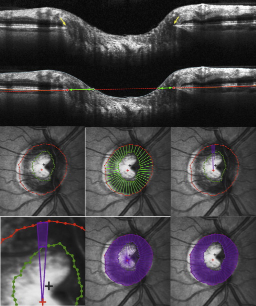
Optical Coherence Tomography Parameterization

The horizontal rim area was designed to resemble conceptually the parameter CSLO rim area and the current SD-OCT rim assessment and to mimic most closely a clinician’s rim assessment. It was based on the distance from the BMO to the inner limiting membrane along the plane of the BMO within each radial B-scan (horizontal), as indicated by the green arrows in Figure 1 . This gives 48 horizontal rim-width measurements (2 for each of the 24 delineated B-scans). For each of these measurements, the corresponding area was calculated using a circular section 7.5 degrees wide and an appropriate diameter, r (based on the distance from the BMO centroid to the BMO in that radial B-scan), as shown by the green outline in Figure 1 . Specifically, the sectoral horizontal rim area equals the difference between the areas of two 7.5 degree circular sectors, one of radius r and one of radius (r – horizontal rim width). These sectoral areas were added to give the overall horizontal rim area measure. For eyes in which the cup was so shallow that the inner limiting membrane never crossed the plane of the BMO, the horizontal rim area was set to equal the entire area enclosed by the BMO. This measure is similar to the rim area measure produced by the Cirrus SD-OCT research software, which performs the same calculation using a reference plane 200 μm anterior to the BMO. BMO points from locations around the optic nerve head generally do not all lie within a single plane (unlike the single depth used to define the CSLO reference plane), but instead form a 3-dimensional elliptical ring with varying axial depths.

The BMO-MRW was based on the distance from the delineated BMO point to the closest point on the inner limiting membrane within each radial B-scan, as first described by Povazay and associates and as indicated by the yellow arrows in Figure 2 . This minimum will occur at an angle θ to the BMO plane (as marked in blue) that can vary between the different radial scans in a given eye. Note that this represents the MWR from each delineated BMO point within 1 side of the radial B-scan, within the plane of the acquired B-scan rather than the global minimum distance to the inner limiting membrane from that BMO location (which would require interpolation of the inner limiting membrane surface between the available B-scans). These rim widths were then averaged across sectors to give the global measure BMO-MRW.

Definition and calculation of the Bruch membrane opening minimum rim width and minimum rim area, as used to estimate the amount of neuroretinal rim tissue in glaucoma (top). Within each of the 24 radial scans, the Bruch membrane opening was delineated (red circles). The minimum rim width within that sector was defined as the shortest distance from this point to the inner limiting membrane (yellow arrow, at angle θ above the Bruch membrane opening plane). These were averaged across sectors to give the global measure of the Bruch membrane opening minimum rim width (middle panel). Within each sector, rim areas (yellow trapezoids) were calculated as the areas of trapezia at varying angles above the Bruch membrane opening plane. The height of each trapezium equals the rim width at this angle, referred to as RW _θ . The base equals the circumference within that sector, 2πr/48, where r represents the distance from the Bruch membrane opening centroid (red cross). The top then has length 2πr / 48 × (r − RW _θ * cos(θ)) (bottom panel). Within each sector, the smallest such area was found, at angle φ, and its area calculated as (top + bottom) × RW _φ /2. Note that RWφ will not always be the minimum rim width within this sector, as illustrated in Supplementary Figure S1 . The global measure BMO-MRA is generated by summing the areas of these 48 trapeziums.

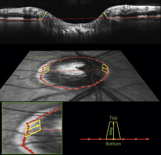
The motivation for assessing this minimum distance is that it approximates the smallest cross-sectional area through which nerve fibers must pass en route from the retina to the optic nerve for a particular part of the optic nerve head. However, it does not provide a true surrogate measure for the number of axons because the same BMO-MRW would correspond to a larger cross-sectional area in eyes with larger discs. Thus, the number of axons would likely better correlate with the minimum cross-sectional area (BMO-MRA) through which the axons pass than with BMO-MRW.

BMO-MRA was estimated as the sum of the areas of 48 trapeziums, each extending from a delineated BMO point to the inner limiting membrane at angle φ above the BMO plane, as indicated by the yellow outlines in Figure 2 . One such trapezium is associated with each delineated BMO point, defined as being at radius r from the BMO centroid. The base of the trapezium then extends halfway to the adjacent radials, so it has a length of 2πr/48. The height of the trapezium is set to equal the rim width at angle φ above the BMO plane in that radial, RW _φ , as shown by the yellow arrows in Figure 2 . The top of the trapezium is then at horizontal distance (r − RW _φ *cos(φ)) from the BMO centroid. This means that the length of the top is given by 2πr/48*(r − RW _φ *cos(φ)). Within each radial, the angle φ was optimized to give the smallest rim area. This means that φ does not necessarily equal θ, the angle of the MRW measurement. They are shown as being the same in Figure 2 for simplicity. For example, consider the case where the rim width perpendicular to the BMO plane (ie, φ = 90°) is 100 μm, and the width parallel to the BMO plane (ie, φ = 0°) is 105 μm, with radius r = 1000 μm. The corresponding sectoral area from the above formulas measured perpendicular to the BMO plane is then 13090 μm ² , whereas the area parallel to the BMO plane is 13023 μm ² . In this example, this sector’s contribution to BMO-MRW would be measured at θ = 90 degrees, whereas for BMO-MRA it would be measured at φ = 0 degrees. θ is chosen to minimize the rim width, whereas φ is chosen to minimize the rim area. Supplementary Figure S1 shows a demonstration of this in schematic form. The areas of the sectoral trapeziums were calculated based on these dimensions and added together to give the global minimum rim area measure BMO-MRA. Unlike the horizontal rim area above, these minimum rim measures are not affected by the possibility that the cup may not break than the BMO plane.

The relationship between the mean RNFL thickness and the corresponding cross-sectional area does not depend on the disc circumference, with one being a multiple of the other. Even though we report an RNFL thickness measure, it can be treated the same as an area measure, in particular allowing the relationship between the RNFL thickness and the rim area to be modeled using a linear fit. We chose to use RNFL thickness because it has been more commonly used in the literature, whether using temporal domain or (as in this study) or SD-OCT.

Data Analysis

The primary outcome measures were the correlations between each of the neuroretinal rim measures (CSLO rim area, horizontal rim area, BMO-MRW, and BMO-MRA) and either RNFL thickness or function (MD). Pearson correlations were used and were compared using the Steiger Z ₂ * test for nonindependent data.

It has been suggested that structure and function are better correlated when the functional measures are expressed on a linear, rather than a logarithmic (dB) scale. Therefore, this analysis was repeated after transforming the functional data onto a linear scale proportional to 1/Contrast. To achieve this, pointwise total deviation values (TD) were converted to 10 ^TD/10 , and then these values were averaged to give the index linearized MD. We have previously reported that this transformation may exaggerate variability at locations with above-normal sensitivities. Therefore, another index was calculated in the same manner after first capping all TD values at zero, capped linearized MD = mean (10 ^{min(TD, 0)/10} ).